Implications of a 5D Entanglement Mechanism for Macroscopic Biophysics Volume 65- Issue 4

Alexander Harrison*

• Fmr Prof of Engineering, The University of Newcastle NSW 2308, Berkeley Computational Research, Berkeley Vale, NSW 2261, Australia

Received: May 04, 2026; Published: May 21, 2026

*Corresponding author: Alexander Harrison, FRSN, PhD, Fmr Prof of Engineering, The University of Newcastle NSW 2308, Berkeley Computational Research, Berkeley Vale, NSW 2261, Australia

DOI: 10.26717/BJSTR.2026.65.010239

Abstract PDF

ABSTRACT

Biological beings are made of fundamental particles that obey laws of quantum mechanics (QM). All matter in 4D spacetime carries a charge either due to electrons, other particles or atoms. Kaluza-Klein (KK) showed that charge results from a particle’s momentum in the fifth dimension (5D), indicating that charged 4D objects exist in 5D. Standard 4D spacetime fails to explain rapid non-local synchronization in large atomic assemblages. A bulk space model in 5D is devised that proves a shortcut for 4D spatial connection as a requisite for quantum entanglement (QE). The resulting mechanism explains how QE works using quantum state operators that connect two particles, while delivering a measurable correlation. No QM violations are evident with this entanglement mechanism. Constraints established by Born, Bell and Lorentz, while proving falsifiable tests, causality and no faster-than-light (FTL) signalling are satisfied. A higher-dimensional geometric mechanism of quantum entanglement extends from particles to macroscopic biological objects that only require the definition of a universal state density matrix Ŝ. Quantum states encoded through a nonlocal τ-space are detectable in 4D with a correlation function to prove entanglement. Implications for biophysics and human non-local interactions are significant, including application to biomedical and measurement instrumentation.

Keywords: Biophysics; Higher Dimensions; Charge, Non-Local Correlations; Quantum Entanglement; Constraints; QM; Causality; 5D Scalar Field; Kaluza-Klein Theory; Born and Bell Rules; Falsifiability; FTL

Abbreviations: QM: Quantum Mechanics; KK: Kaluza-Klein; QE: Quantum Entanglement; FTL: Faster-Than- Light; 5D: Fifth Dimension

Introduction

All biological processes operate with charge as the fundamental electrostatic carrier of information. Charge is the basis of life forms and their biology. Neural signals are ionic charges that flow using Na⁺, K⁺, Ca²⁺ ions. DNA itself is charged base pairs held by H-bonds, while protein folding is purely due to electrostatic interactions between charged residues. At a cellular level, cell membranes contain charge separation across lipid bilayers, and consciousness is also assumed to be ultimately electrochemical, i.e., charge-based. Linking these known physiological facts to an underlying quantum mechanism is not academic. Many medical devices currently use quantum-based technologies, ranging from bio-medical equipment, solid-state devices and portable electronics, applied radiation isotopes, alternative energy photovoltaics, scanning nuclear technologies, telecommunications, aviation and advanced computers. A broader understanding of quantum physics has invariably led to the widespread application of new discoveries. Continual development of quantum-based devices, especially in the biomedical field, relies on physics research. In this regard, new understanding of quantum mechanisms will become viable for technical innovation.

Between 1921 and 1926, Kaluza-Klein (KK) derived a unified electromagnetism-gravitation theory functioning in the 5D bulk space τ. KK showed that Fifth-dimensional momentum has charge as its eigenvalues [1-6]. The KK charge literally encodes quantized τ oscillations of the entanglement correlation around the 5D manifold. In 4D spacetime, measurements show spatially separated particles can share the same quantum states described as quantum entanglement (QE), however the “how” is missing from the QM model. All biological entities already participate in the τ dimension by virtue of being charge-based. A human being is not separate from τ, rather a 5D object whose 4D projection involves charge, quantum states, and neural processes. As will be shown by proving a τ-dimension quantum entanglement mechanism in this paper, particles and atoms including cells are described by a quantum state operator Ŝ, which is a real-valued density matrix. One does not need to ask about the τ-component of the total quantum state Ŝ of a person; the component already exists due to charge.

An analogy is that an electron has a charge e– and its external electric field is not injected into the τ-space around the particle, the electric field Ē simply exists because of the electron charge. When humans learn how to manipulate nonlocal-based information, unknown technologies will emerge. First, the basis of the information “flow” in the τ-dimension needs to be established by proof, which is set out in this paper. A short history of the background of quantum mechanics is important in context. In over 100 years no mechanism describing how particles become state-entangled is known, as if the QM model is sealed to any other solution due to constraints placed on any alternative model. As a conjecture, this may be why human development in relation to gravity, precognition and other “feeling related observations have no proven mechanism to date.

Nonlocal Quantum Biophysic

A test of any new QE mechanism should in principle be scale-independent. A human body is a 4D quantum system consisting of approximately 7 × 10²⁷ atoms. Each atom has quantum states. Each electron, proton, and neutron has a quantum state describable by some density matrix Ŝ [7]. In principle, the total quantum state of a human body B is Ŝ_B = |Ψ_B⟩⟨Ψ_B|, a density matrix of astronomically large size. It is still a valid density matrix of exactly the same mathematical form as Ŝ for a single electron which has a 2x2 spin matrix. In reality, superposition of all quantum states k involves summing Ŝ states, mathematically expressible by Ŝ_T = Σ_k W_k |ψ_k⟩⟨ψk| where Ŝ_T is a mixed state density matrix and the sum runs over each particle “k” in the person’s body, and Wk are state weights. Quantum state Ŝ_t is completely valid in quantum mechanics. No reason exists why Ŝ_T would not exhibit a charge value, no matter how small, meaning its presence already exists 5D. By extension, all biological entities exist in 5D space via their charge, based on the KK theory, further suggesting all matter has a 5D existence in a M5 manifold. For analysis, define a 5D coordinate as X = (x, y, z, t, τ), containing every 4D hypersurface as submanifolds. Every object has its own hypersurface at τ = τ₀, one particular slice of the 5D space. In quantum mechanical terminology, this realization means that any two particles or persons such as P1 and P2 have quantum density matrices Ŝ₁ and Ŝ₂, respectively.

At a particle level, its quantum state operator is a real density state matrix, Ŝ, whose value exists as an intrinsic property of the quantum state of P1 or P2. As described in the following sections, charge components also exist in a 5D scalar field Q(x, y, z, t, τ). Field Q is expressing its natural 5D character on the slice where it exists, and the 5D field Q extends that character to other points in M5, including the location of P1 on the same or neighboring τ-slice. No information flows or crosses a boundary, nothing is injected across a gap, it exists. In terms of writing a proof, the 5D field value at P1 is not caused by something sent from P2, rather by the intrinsic 5D character of P2’s quantum state. This state is defined as a charge in the deepest Kaluza-Klein sense, extending through the 5D space that both P1 and P2 already inhabit. All charged particles and objects with a positive Ŝ are quantum systems that are natural participants in τ without any additional mechanism. State Ŝ does not reach into τ, Ŝ already as a 5D object [7].

Model Constraints

Quantum mechanics (QM) began in the early 1900’s with the work of notable scientists such as Plank, Heisenberg, Born and Schrodinger. Over the last century, significant technological applications of quantum physics have emerged in society. Quantum entanglement (QE) theory began in 1935 with the work of Einstein, Podolsky and Rosen, during attempts to prove QM incomplete. In 1964 Bell devised a testing theorem for entanglement, to later be experimentally verified in the 1970’s by Aspect. Literature on quantum entanglement is extensive [8-11]. In 2022, Aspect, Clauser and Zillinger won the Nobel Prize in Physics for their work on QE’s existence, even though no valid mechanism existed. Whilst quantum entanglement correlation has been verified by measurements over the last 50 years, a clear proof is missing from the QM theory of an exact mechanism of how QE occurs.

Experiments confirm that measuring one particle of an entangled pair instantaneously determines the correlated state of the other particle, regardless of distance between them, but the “how” is unknown. Earlier research using a nonlocal field investigated use of 5D to describe a mechanism for precognition and nonlocal cognitive interaction. Similar methodologies are used in this current work to further investigate quantum particle entanglement. A fundamental question arises as to how two spatially distant biological beings sense future events [7]. Even more fundamentally, how are particle states linked by quantum entanglement? Hints exist in the physics literature about fields. Kaluza-Klein’s theory (KK) considered a 5D framework to unify gravity and electromagnetism [5,6]. KK argued that by adding a 5th dimension τ, a scalar field might emerge from this compactification of space [7]. For the want of a name, the dilaton or radion field was postulated. In 1926 Born devised a rule to prove the probability of a particle’s existence at a stated location [7]. Entangled particle theories cannot violate quantum mechanical constraints. Constraints exist and are consequential to the development of new mechanisms that might explain how quantum entanglement works. A QE mechanism must not violate the following six QM “Constraints”;

1. Born Rule: The probability density P of measuring a quantum entity is P = |ψ|² [7].

2. Bell Inequality: QE has a stronger statistical correlation than shown in classical models [2].

3. No FTL: No faster-than-light (FTL) information flow, no signaling [8,9].

4. Lorentz Invariance: Physics must be invariant in all frames of reference [11].

5. Causality: Effect must not precede its cause [10].

6. Experimental Falsifiability: A testable prediction that differs from QM [2].

A scalar field mechanism for entanglement has been investigated in other areas of research describing non-local cognitive interactions [7,12]. where biological entanglement is demonstrated. In that research, a bulk fifth-dimension scalar field containing an information state can be detected to prove state entanglement correlation without violating causality and FTL action.

Quantum Entanglement Mechanism

As a natural progression of previous research, analysis of a two-particle system for entangled states needs to consider their quantum mechanical constraints in considerable detail. Recent research related to QE is widely recognized [13-21]. Solving how QE works would be a significant result because the underlying mechanism is genuinely unknown. An entanglement model consists of real particles P1 and P2 described with a 5D τ-component of their quantum states. As shown by the KK unified electromagnetic and gravitational field theory, electric charge in 4D results from a particle’s 5D momentum, i.e. motion in the fifth dimension τ, as a basic τ-dimension phenomenon projected into 4D [5,6]. More specifically, charge is the natural source by which 4D quantum states exist in a fifth τ dimension, allowing quantum state statistics from one particle to be nonlocally available anywhere in τ.

Mechanism and its Geometry

Coordinate X = (x, y, z, t, τ) is a free variable in 5D bulk space. Particles P1 and P2 have coordinates X₁ = (x₁, y₁, z₁, t₁, τ₁) and X₂ = (x₂, y₂, z₂, t₂, τ₂), respectively. For analysis, particle P₂ is measured first at time t₂ (the cause) with quantum states available at P1 (the effect) through the Q field, i.e. t₂ < t₁ and (t₁ – t₂) > 0 is always valid [validates Constraint 5]. A quantum state operator, Ŝ₂, contains P2’s quantum statistics, such as real valued spin matrix or a general density matrix. P2’s fixed coordinate X₂ is pinned in place by Dirac delta functions which also pins the τ-component of P2’s quantum state in the 5D scaler field Q. A quantum state amplitude of Ŝ2 exists at P1’s location X₁ that holds P₁ to a fixed t₁ and τ₁ coordinate. Evaluation of Q at P1’s location X₁ requires the computation of Q(X₁) by solving a 5D field equation containing a retarded Green’s function G^R5(X, X’). P2’s statistics in the 5D bulk exists at P1’s hypersurface and is available for detection at P1 by a sampling function I₁(t). Finally, a detection statistic R₁(t) > s, where s is a threshold trigger, giving the entanglement correlation of the state of P2 at P1.

5D Minkowski Interval

Small-interval ds² = gμv dxμ dxv + φ(x)²dτ² exists in the curved 5D bulk manifold, where gμv is the 4D spacetime distance and φ(x) is dilaton scalar field (can vary with position) [22]. Dilaton field φ encodes the size of the τ dimension at each point in 4D spacetime [5,6]. Flat space approximation by the 5D Minkowski is ds² = [ − dt² + dx² + dy² + dz² + dτ² ], or its equivalent Euclidean length is D = − Δt2+ |Δx|2 + (Δτ)S [23]. Spatial separation of particle’s P1 to P2 is |Δx| = |x1 – x2|, with y and z left off for brevity. As length |Δx| → ∞, connection is only possible through the τ dimension rather than across the 3D spatial separation. In 5D space, ||Δx| is not considered, so D = [ – Δt² + 0 + Δτ²]. When Δτ ~ Δt, the 5D path length D ~ 0; a geometric bulk “shortcut” independent of ||Δx| in 4D spacetime. Lorentz’s invariance is not violated because τ is a 4D [Constraint 4 satisfied].

5D Field Equation Solution

A scalar field Q(X) = Q(x, y, z, t, τ) is defined over all fifth-dimensional space. Using a Klein-Gordon wave equation, driven by a quantum source operator Ĵ_P2(X), a non-homogeneous pde describing the field Q at any coordinate X in 5D is [6,22];

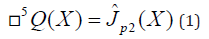
where ◻⁵ is a 5-axis d’Alembertian wave operator [23], and ĴP₂(X) is a quantum source event operator containing Ŝ₂. Dirac delta functions (see following sections) enforce ĴP₂ = 0 everywhere except at X = X₂. The field amplitude of Q that P1 experiences due to P2’s measurement is Q(X₁) at X₁. Equation (1) has a solution for Q(X₁) at P1 requiring five integrals [17,24];

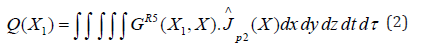
with the free variable X ranging over every point in 5D space. A bi-local retarded Greens function G^R5(X₁, X) in the solution represents the “free” charged part of Q(X₁) evaluated at P1. Evaluation G^R5(X₁, X₂) becomes the “fixed” charged part because it specifically evaluates G^R5 at P2 and P1. Calculation of G^R5(X₁, X₂) is therefore required. Defining Ĵ_P2(X) is carried out before present a solution to G^R5 for flow of the model solution. Source Ĵ_P2(X) consists of both Ŝ2 and Dirac delta function switches which pin P2 at X₂ to 4D and 5D coordinates so that Q can be properly evaluated at X₁. A discussion on Dirac delta functions provides some useful background [25].

Source and 5D Propagator Functions

Quantum entanglement between particles P1 and P2 requires a solution to the field Q(X₁) at P1. Let quantum state operator Ĵ_P2(X) be a field equation source that contains P2’s statistics Ŝ2, where P2’s position is known absolutely. Using Dirac delta functions to pin Ŝ2 to P2’s coordinates exactly at X₂ = (x₂, y₂, z₂, t₂, τ₂), and by linearity, abbreviate (x, y, z) in (x) only for brevity;

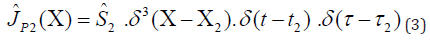
which means the exact location of P2 is known only when X = X₂. The integral in Equ. (2) fires with P2 evaluated giving Ĵ_P2(X) = Ŝ2. Everywhere that X ≠ X₂ and Ĵ_P2 = 0. In Equ. (3), Dirac delta functions force P2’s location exactly at its X₂ coordinates and force the probability of finding P2 at X₂ as P = 1, consistent with the Born rule [validates Constraint 1]. As a result, there’s no premature signal and no FTL signaling [validates Constraint 3]. Green’s function connects two objects [17]. A bi-local retarded Green’s function acts as a 5D propagator between source P2 and detector at P1. Inside the integral of Equ. (2), Dirac delta functions contained in Ĵ_P2(X) have been adopted and used to ensure that Equ. (3) collapses X to X₂. Inside the integral;

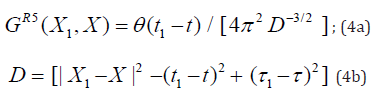
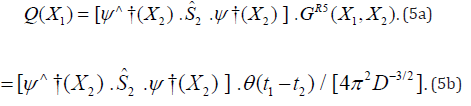
with θ(t₁ − t) a Heaviside step function θ(t) used as a switch to ensure time causality in the model, having a value θ(t₁ − t) = 1 when t₁ > t (effect after cause) while θ(t₁ − t) = 0 when t₁ < t (blocks retro-causality). After the integral fires in Equ. (2), at X = X2, and the retarded Green’s function is evaluated, G^R5(X₁, X2) = θ(t₁ – t₂) / [4π² D-3/2], where θ(t₁ − t₂) = 1 only when t₁ > t₂. Since P2 is always measured first, θ = 1, hence G^R5 is the retarded propagator. Length D = |Δx|² − Δt₂+ (Δτ)² where |Δx| = |x1 – x2| is the 3D spatial separation (can be large and non-zero), Δt = (t₁ – t₂) >0 is the temporal separation (always positive) and Δτ = (τ₁ − τ₂) is the 5th dimension separation. With regard to established quantum field theory (QFT) [26], Equ. (3) should be clarified for completeness. While Equ. (3) is sufficient and works as intended, the expectation ⟨Ĵ2P⟩ = 0 before measurement at P2 makes Ĵ_P2 a natural consequence within QFT rather than an assumption. In this case, Ŝ₂ in Equ. (3) could be replaced by {ψ⌃†(X) ⋅ Ŝ₂ ⋅ ψ⌃(X)} where quantum field operator ψ⌃†(X) creates (adds) a particle’s existence at X, while ψ⌃(X) annihilates (reads) the particle at X. In other words, ψ⌃(X) tests or asks if a particle exists at X, so ψ⌃(X) will remove a particle at X, while ψ⌃†(X) puts it back at X. If there is no particle at X, ψ⌃(X) · |vacuum⟩ = 0; there’s nothing to remove.

Simplifying Equ. (3) with δ5(X – X2) = δ³(x – x2) · δ(t – t₂) · δ(τ – τ2), the source operator J becomes Ĵ_P2(X) = ψ⌃†(X) ⋅ Ŝ₂ ⋅ ψ⌃(X) · δ5(X-X2) which complies fully with QFT [27]. Modifications of Equ. (3) to include quantum field operators makes the model fit fully inside QFT where all interactions are written in terms of field operators. Measurement of a particle’s density number ŵ(X) = ψ⌃†(X) · ψ⌃(X) is a first test for existence. If the value of ŵ(X) = 0 then there’s no particle at X, or if ŵ(X) = 1, a particle definitely exists at X. Adding the 5D Dirac delta switches used in Equ. (3) produces the full form for the quantum source field operator Ĵ_P2(X). More importantly ŵ(X) places all actions inside QFT, and not by just assuming that Ĵ_P2 = 0 when X = X₂. Equation (2) results in a full QFT-valid field description at X₁ when the integrals fire at X₂, i.e.;

G^R5(X₁, X₂) is non-zero for all values of |Δx|, however large. Entanglement correlation does not decay with distance. Causality [Constraint 5] is not violated because θ(t₁ – t₂) = 1 only when t₁ > t₂. The Lorentz requirement [Constraint 4] is not violated because τ is a scalar and Δτ does not break the 4D Lorentz covariance. A probability P of detecting a correlated state between P2 and P1in 5D space is P ∝ | G^R5(X₁, X₂) |² · |⟨Ŝ₂⟩|², where ⟨Ŝ₂⟩ is the expectation value of Ŝ2 and |⟨Ŝ₂⟩|² is the Born probability of P2’s state. Here the universal quantum state density matrix Ŝ₂ contains all P2’s Born statistics for P1 and acts causally via G^R5(X₁, X₂) [validates Constraints 1, 4, 5].

About P2’s State Operator

Recall that particle P2 maybe any particle type with any observable. Operator Ŝ₂ can be considered a universal form for all particles. Measurement of a quantum particle affects the particle’s state, so at the moment P2 is measured, Ŝ₂ is the pure-state density matrix representing the state of particle P2. Density matrix Ŝ₂ is defined by Ŝ₂ = |ψ2⟩⟨ψ2|, where |ψ2⟩ defines the quantum state of P₂ and is a column vector in Hilbert space while ⟨ψ2| is the conjugate transpose of |ψ2⟩ in the matrix, as a row vector. Describing the Ŝ₂ matrix in Hilbert space allows for infinite dimensions and a geometry with angles and lengths, an ideal space for quantum mechanical analyses [28]. Because Ŝ₂ is purely a universal quantum state amplitude, its validity is unquestioned but Ŝ₂ needs a τ-component in bulk space; achieved by placing it in J(X) as part of the Q field. All of P2’s states then satisfy Born probability statistics [validates Constraint 1] and since Ŝ₂ is a global bi-local quantity with no hidden variables at P2, Bells locality assumption is inapplicable and sidestepped [validates Constraint 2].

Falsifiability Test Argument

The 5D bulk path D = [−Δt₂+ |Δx|² + (Δτ)² ]. Without a 3D component, is D = ( − Δt² + Δτ² ) which is small if Δτ ~ Δt. Suppose that both Δt and |Δx| grow in slightly different but small ways in τ space. For small parameters α > 1 and β ∈ ℝ, let Δτ = (τ₂ − τ₁) = α·Δt + β |Δx|, so that D becomes;

If D* > 0 always then α > 1 is necessary and sufficient, meaning that for Δτ = α·Δt + β |Δx|, the derivative dτ/dt = α along worldlines, meaning that τ grows faster than t, and thereby creates the geometric bulk shortcut through the 5D manifold. For β real, τ also tracks |Δx| spatial separation while G^R5 is non-zero at all distances, i.e. distance independent. Therefore, small coefficient α·adjusts Δt as τ evolves. Since α >1, let it be defined by α = (1 + ε) as a correction where ε > 0. A specific experimental method to measure ε is a project for laboratories. Falsifiability requires that the model makes at least one prediction which differs from standard quantum mechanics. Standard QM has no τ dimension or ε parameter to allow proof of quantum entanglement. Standard QM predicts ε does not exist. This model predicts ε does exist because α > 1, i.e. α = (1 + ε), which implies ε > 0. This is a different prediction from standard quantum mechanics and therefore the falsifiable constraint is not violated [validates Constraint 6]. Detecting Entanglement at P1

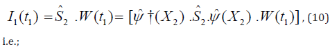
In an analogous way to how Equ. (2) is formed, detection of P2’s state at P1 works as an information extraction and correlation process from the 5D field Q. An exception is that the extraction equation has to be pinned to P1 using a spatial sampling integral as a classical field form of the field Q at P1’s measurement time t₁. A sampling integral is defined by I₁(t₁), a classical field sampling of the field Q in which the quantum content of P2 via Ŝ₂ naturally and completely exists. A physical detector at P1 responds to the field Q in its neighbourhood, not by measuring Q at a single point, rather measuring a weighted average of Q over the spatial and τ region it occupies;

which is a spatial sampling integral where w(x, τ) is a window function centered on P1, weighting nearby field values more than distant ones. Substituting I₁(t₁) for the observed point X* = (x, t₁, τ) rather than the single fixed point X₁, into the evaluated field Q(X₁) = Ŝ₂ ⋅ GR5(X₁, X₂), gives;

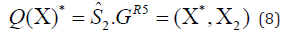
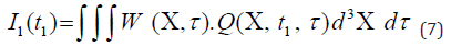
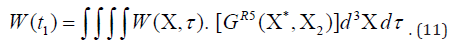
and substituting into the sampling integral gives the classical field integral Equ. (7);

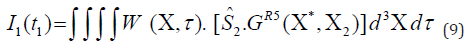
Noting that Ŝ₂ is fixed at location X₂ of P2, it moves outside the integral. Letting W(t₁) be the geometric weight integral, Equ. (9) simplified to;

Geometric factor |W(t₁)|² is the classical field intensity at P1, non-zero for all |Δx| and is the spatial average of |G^R5|². Detector output value is then defined by;

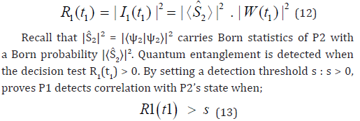
In reality |W(t₁)|² represents geometric detection efficiency, an indicator of how much of the 5D field Q actually reaches P1’s detector window. The amount depends on the shape of w(x, τ), how broadly P1 is sampled, the value of GR5 which depends on |Δx|, Δt, Δτ, and parameters α and β. In addition, |W(t₁)|2 is a classical geometric amplitude. Quantum probability P = |⟨Ŝ₂⟩|² depends on ⟨Ŝ₂⟩, the expectation value of Ŝ₂. Correlation observed at P1 through R₁(t₁) inherits Born statistics through the quantum state operator Ŝ₂ embedded in Ĵ_P2(X). A probability weighting at P1 is consistent with the Born rule without requiring separate postulates within the 5D framework and satisfies that consistency requirement.

Table of Findings

Compliance results for a nonlocal quantum entanglement mechanism shows where and which constraints apply in Table 1. When a constraint is not violated in Table 1, it is designated as “Comply”, whereas multiple constraints are labelled as “Complies”. Constraint number “No.” in the table are taken from the six requirements in the Introduction. Connecting person P1 to Person P2 with an information state Ŝ₂ realized by person P2 is the same as the quantum entanglement mechanism between two quantum particles. The idea that the quantum entanglement process can be scaled to human and biological systems is a profound concept because the implications for human interconnection will change the way humans feel each other’s existence. While Table 1 shows the steps between P2 and P1, as will be discussed in the next section the extension to large organisms is mathematically sound though futuristic relative to current technology.

Bio-Significance of QE

Development of a verifiable mechanism that proves quantum entanglement at a particle level has significant implications for human and biological interaction. Scientific understanding that quantum particles can entangle across great distances and share states implies that any complex biological entity can nonlocally interact using the total residual charge that is naturally embedded in 5D. Since all biological processes have a τ-connection due to charge, the question is not whether minds can access 5D, they already do by virtue of charge. A person’s mind is automatically resident in a 5D manifold and the mechanism shows how it is accessible in the field Q. A logical extension of the findings leads to a discussion about what the τ-component of a conscious quantum state is in practice, which will lead to new research programs. Proof of particle entanglement at a quantum level solidifies a pervasiveness that underlies macroscopic human effects such as premonition, telepathy and precognition. Applying the model to human interaction uses the charge metaphor as a real 4D measurable effect at a physics level, based on the KK analysis which has never been disproven. By the QE mechanism described above, a person’s P2 quantum state Ŝ₂ charges the 5D scalar field Q at its location X2. Charging requires no transmission, no sending, no injection into 5D, is the natural expression of P2’s quantum state amplitude in the 5D space that P1and P2 both inhabit. The field value Q(X₁) at P1’s location is not received from P2, it exists as the natural 5D extension of P2’s quantum charge, propagated geometrically in the τ bulk manifold via G^R5(X₁, X₂).

Wording such as “propagate” is misleading in this context because it implies a motion, however a better description is that charge pervades 5D space without delay and irrespective of light-speed in 4D. This is consistent with Kaluza-Klein where charge is literally momentum the 5th dimension, where 4D reality already exists within 5D. A fundamental insight now exists, that the question of how to reach τ simply dissolves. Based on the model, an equivalent macro-state of person P2 is already known in 5D because of their density state matrix Ŝ₂, no matter how large. Density state Ŝ₂ does not reach into τ in some nebulous way, Ŝ₂ is already a 5D object whose τ-component exists in J_P2(X). Quantum entanglement connects premonition, telepathy and precognition research in the most natural way. The general 5D QE mechanism is scale-independent. In the Introduction, a human body is a quantum system of charge if one considers it consists of somewhere near ~ 1028 atoms. Each atom has quantum states. Each electron, proton, and neutron has a quantum state describable by some density matrix Ŝ. Already indicated, the total quantum state of a human body B is ŜB = |ΨB⟩⟨ΨB|, the density matrix of astronomically large dimension but it is still a valid density matrix.

Practical considerations do exist with analysis of QM applied to a human body, however future technology could resolve issues such as decoherence. Decoherence is where short-lived quantum states of individual particles in a warm, wet biological system decohere, i.e., they lose their quantum nature and become classical. In classical terms, biological effects occur at known time constants, so a single electron spin decays in ~10-13 seconds, a molecule vibration state exists for ~10-12 seconds, while a human neural process takes a milli- second. This means that the off-diagonal coherence terms in the large Ŝ₂ matrix that carry quantum information will collapse to zero almost instantaneously in biological tissue. What remains is a classical probability distribution, not a quantum state. The entanglement mechanism in this model requires the coherence terms to survive long enough to be part of G^R5. Whether those small coherence terms are sufficient for G^R5 to provide a detectable signal to another person is an open quantitative measurement by finding ε and s values in the QE mechanism.

Nonlocal Human Correlation

If quantum coherence persists in some subset of biological processes, even briefly, then in principle Ŝ_B at time t₂ (a future event) could source ĴB(X) which expands in Q with G^R5(X₁, X₂) to another person P1 at time t₁ < t₂. This would be the 5D geometric mechanism for what phenomenologically appears as nonlocal human correlation and information transfer as described in Table 2. In describing these human interactions, the mathematics does not forbid them. The 5D model does not contain any equation that says the mechanism only works for simple two-state particles and not for complex biological systems. However, three issues currently separate these observations from being a full scientific claim;

1. Decoherence is a question because no experimental evidence exists to date that quantum coherence persists at the scale needed in biological neural tissue. Atomic charge decoherence become irrelevant with a 5D mechanism since it is bypassed.

2. The signal strength used in the detection threshold s in R₁(t₁) > s would need to be extraordinarily sensitive to detect a signal from 1028 partially decohered quantum states at macroscopic distance. Measurement instrumentation will be developed.

3. Experimental validation that premonition and precognition research papers would need to demonstrate that the observed effects scale with the predictions of the 5D model, specifically the shortcut finding, where (1 + ε) is measurable for human bodies.

From a physics perspective, the model establishes the 5D mechanism for quantum entanglement between particles and proves that the six QM constraints are satisfied while making a falsifiable prediction that ε and β corrections are measurable. The model allows a discussion of biological neural states that possess sufficient quantum coherence to constitute a valid ŜB operator, which is testable alongside an empirical question about decoherence times in neural tissue. At a phenomenological level, research provides the observational data and documented cases of precognition, telepathy, premonition. These become the R₁(t₁) > s detections in the biological regime. If the statistics of premonition data match the predicted distribution from the 5D model, particularly the distance independence and the temporal ordering, such measurements would be extraordinary evidence that macro-scaling of quantum entanglement is valid.

Conclusion

Entanglement of two quantum particles separated in 4D space is described by a nonlocal mechanism that is proven to comply with the six QM constraints of quantum mechanics. Extension of the new mechanism to larger biological entities like human beings is physically realistic. Quantum particle entanglement is well-documented at the subatomic and atomic levels. Current QM models are unable to account for macroscopic coherence in complex biological systems. Standard 4D spacetime constraints fail to explain rapid non-local synchronization observed in large atomic assemblages such as human physiology. This paper shows how a 5D geometric framework allows for entanglement states that bypass traditional decoherence, providing a basis for biological unity. By extending the entanglement manifold into the fifth dimension, residual atomic charge between human bodies allows instantaneous transfer of information that’s not possible within a strictly 4D relativistic framework.

With a correct 5D mechanism proving how quantum particle entanglement functions, extension to biological systems simply requires that a sufficient quantum coherence persist in human neural processes to constitute a valid ŜB matrix value that can source ĴB(X). The paper shows that a measurable time-related parameter ε exists, implying 5D space is real. In addition, the fact that nonlocal precognitive effects are known in human society means that the 5D model has a plausible application. Premonition and precognition research, along with this physics model, describe the same underlying mechanism at different scales. The physics simply requires coherence data to prove scaled up QE effects for people, from which the calculation of signal detectability is made per a R₁(t₁) > s measurement and an ε value such that ε > 0.

References

1. Aspect A, Dalibard J, Roger G (1982) Experimental test of Bell’s inequalities using time varying analyzers. Physical Review Letters 49(25): 1804-1807.
2. Bell J S (1964) On the Einstein Podolsky Rozen paradox. Physics Physique Fizika 1(3): 195-200.
3. Bouwmeester D, Pan J W, Mattle K, Eibl M, Weinfurter H, et al. (1997) Experimental quantum teleportation. Nature 390(6660): 575-579.
4. Hensen B, Bernien H, Dréau A E, A Reisereret, N Kalb, et al. (2015) Loophole free Bell inequality violation using electron spins separated by 1.3 kilometres. Nature 526(7575): 682-686.
5. Kaluza T (1921) Zum Unitätsproblem der Physik. Sitzungsber Preuss Akad Wiss 1921(1921): 966-972.
6. Klein O (1926) Quantum theory and five dimensional relativity. Z Phys 37(12): 895-906.
7. Born M (1926) Zur Quantenmechanik der Stoßvorgä Zeitschrift für Physik 37(12): 863-867.
8. Harrison A (2026) A mathematical theory of precognition. 4th Int. Congress Behavioral & Social Science Research (ICBSSR), Mar Rome Italy, p. 23-24
9. Ghirardi G C, Rimini A, Weber T (1980) A general argument against superluminal transmission through the quantum mechanical measurement process. Lettere al Nuovo Cimento 27(10): 293-298.
10. Riggs P J (2009) Quantum causality: conceptual issues in theory of quantum mechanics. Dordrecht; London: Springer. Available from the State Library of NSW (N530.12/79).
11. Lorentz inequality Bell J S (1964) On the Einstein–Podolsky–Rosen paradox. Physics 1(3): 195-200.
12. Harrison A (2025) Human premonitions explained by nonlocal entanglement theory. UAR J Multidisciplinary Studies 1(8): 1-18
13. Randall L, Sundrum R (1999) An alternative to compactification. Phys Rev Let 83 (1999): 4690-4693.
14. de Broglie L (1924) Recherches sur la théorie des quanta. Annales de Physique 3(10) : 22-128.
15. Maldacena J, Susskind L (2013) Cool horizons for entangled black holes. Fortschritte der Physik 61(9): 781-811.
16. Y D Chong, Y D (2021) Green’s functions, Complex Methods for the Sciences. MH2801. Nanyang Technological University.
17. Douhou A, Ennadifi S E, Jebli N (2019) Quantum entanglement through hidden dimensions. Journal of High Energy Physics, (7), Article 123.
18. Dietrich A, Been W (2003) An Extra Dimensional Approach of Entanglement.
19. Anon (2025) — "Quantum Entanglement as a Higher-Dimensional Effect of the 5D Time-Field" ResearchGate Preprint.
20. Breban R (2005) Interpretation of the five dimensional quantum propagation of a spinless massless particle. Progress of Theoretical Physics 114(3): 643-668.
21. Boguña M, Krioukov D (2025) Local d’Alembertian operator for causal sets. Phys Rev D.
22. Gordon W (1926) Der Comptoneffekt nach der Schrödingerschen Theorie Z Phys 40(1-2): 117-133.
23. Minkowski H (1909) Raum und zeit [Space and Time]. Phys Z 10: 75-88.
24. Peskin M E, Schroeder D V (1995) "An Introduction to Quantum Field Theory", Westview Press / Perseus Books, ISBN: 978-0-201-50397-5.
25. Stakgold I, Holst M (2011) Green’s Functions and Boundary Value Problems 3^rd (Edn.,), Wiley.
26. Courant R, Hilbert D (1962) Methods of Mathematical Physics (Vol. 2). Wiley Interscience.
27. Giardino S (2026) Self interacting quantum particles and the Dirac delta potential. Brazilian Journal of Physics, 56, Article.
28. Ma Y, Wu J (2018) 5-dimensional Kaluza-Klein Theory with a Source. ArXiv.org., 0311015v4.