info@biomedres.us
+1 (502) 904-2126
One Westbrook Corporate Center, Suite 300, Westchester, IL 60154, USA
Site Map
Received: January 13, 2025; Published: January 24, 2025
*Corresponding author: Shahbano Khan, London Metropolitan University London, United Kingdom
DOI: 10.26717/BJSTR.2025.60.009439
To assist physicians in their care, patient decision support systems are developed and introduced. Usually, they function by medical data processing and a level of knowledge with clinical experience. Improvements to these frameworks will develop the efficiency of medical diagnosis decisions, and the healthcare system is commonly viewed as ‘information-rich’ but ‘knowledge-poor’. Within the healthcare sector, there is a variety of evidence available. However, in order to uncover secret associations and patterns in results, there is a shortage of appropriate research methods. multiple applications in business and science areas have been identified for extracting knowledge machine learning and deep learning. Using machine learning and deep learning methods in the health sector, useful knowledge can be identified. In this study, we thoroughly examine the prospective use of classification-based machine learning and deep learning techniques such as SVM, logistic regression, K-Nearest Neighbour, Extreme Gradient Boost, Random Forest Decision tree, Naïve Bayes, Artificial Neural Network and CNN to massive volume of healthcare data.
The industry in healthcare gathers vast quantities of clinical data that can estimate the risk of patients having heart attack using medical profiles such as age, sex, blood pressure and blood sugar. It helps essential information to be identified, e.g. trends, connexions between medical factors linked to heart disease. The application of machine learning and deep learning approaches in risk assessment models in the clinical area of cardiovascular medicine is presented in this sense. By using machine learning and deep learning approaches in both supervised and unsupervised learning processes, the data is modelled and categorised.
Abbreviations: SVM: Support Vector Machine; RF: Random Forest; KNN: K-Nearest Neighbour; LR: Logistic Regression; CP: Chest Pain; ANN: Artificial Neural Networks
Incentives
Cardiovascular disorder. The most prevalent human disease in the world that poses a danger to life is cardiovascular disease. In this condition, in order to perform the normal features and functionality of the body, the heart is typically unable to pump the necessary volume of blood to all areas of the human body [1]. There are other issues along with cardiovascular disease. Arteriosclerosis, which normally indicates the hardening of the arteries, becomes deeper and inflexible in this situation. Atherosclerosis suggests narrowing of the arteries, so that the build-ups have less blood supply (Varun, Mounika, Sahoo, & Eswaran, 2019). Heart attacks normally occur as blood clots or the blood supply from the heart is blocked Cardiovascular disorders arise when the blood and heart vessels do not properly function [2]. It results in heart disease that is permanent. One of the biggest issues of heart disease is the proper diagnosis and discovery of it inside a human being has created many severe problems. Different diagnostic devices are present on the market to diagnose heart disease, and they’re very costly and not accurate enough to measure the possibility of heart disease. Until diagnosing CVD, various checks are done, some of them seem to be auscultation, ECG, cholesterol blood pressure and sugar in the blood. If the health status of a patient might be vital, these assessments often are lengthy and time-consuming, and he / she needs to start immediate treatment so that it to prioritise the exams, it is important to [3].
There are many health patterns that lead to CVDs, such as, gender, age, blood pressure, smoking, etc.. it is therefore important to recognise which lifestyle habits lead to CVDs in order to be able to practise good health habits. With the advancement of computer technology in numerous research fields, including medical sciences, there is a need to find a stronger and accurate way to diagnosing heart diseases at an early level, which has been achieved with the aid of machine learning and deep learning techniques Owing to an increase in the volume of data, machine learning and deep learning are an emerging trend today. Both learning allows to derive knowledge from a huge amount of very cumbersome details to us and even unthinkable as well [4]. The aim of the research is to emphasise the test for diagnoses to see some of the health patterns that lead to CVD. In addition, and most critically, related algorithms for machine learning and deep learning are correlated according to various execution metrics. Manually categorised data is included in this research. Classification by guideline is either safe or unhealthy. 70 percent of data are supervised or educated based on a learning algorithm approach called classification, and 30 % are evaluated in this thesis. Thus, according to their estimation performance, various algorithms are compared [5].
Problem Statement
The prediction model is best suited because of certain complications associated with therapeutic procedures, such as the delay in the results and the non-availability of medical services to persons. While the prediction model is not an alternative to conventional therapies, it will act as a first-hand method for learning and planning for some form of illness.
Research Aim and Objectives
The purpose of this study is to create models to describe the connection between both the features of the dataset of Cleveland heart disease. Given the intent of this report, the aims for achieving the objective are
I. To transform the Cleveland dataset to form a suitable model for machine and deep learning.
II. From the dataset, review the structure and model parameters.
III. To draw inferences from the model constructed.
IV. To equate the model with the algorithm for machine learning and deep learning.
Expected Contributions
The machine learning and deep learning model is supposed to help draw inferences about heart diseases, thereby acting as a diagnostic platform for medical professionals to assist them [6].
Conceptual Outline
In this section some basic concepts and terminologies, such as machine learning and deep learning classification are covered existing and related works using various techniques on heart disease prediction. For implementation the data collection, method, used and the result and consistency of the procedure was checked, reviewing what has been achieved how it has been achieved the classification process used.
Machine Learning Overview
This field of study came into existence since from 1959 it is the repetitive subfield of computer science which is an escalating topic dramatically in the present and is anticipated to rise up more in the future and coming days with energetic applications and research in the previous past decades such as self-autonomous cars, machine control system, web search effective, face recognition etc. are some few areas where machine learning is been used the world is flooded with lots of data and data is been created rapidly on daily curriculum basis all around the world according to the companies in big data and analytics solution like csc it is been expected that every year the amount of data will be greater compare to the previous years like from 2009 to 2020 the data becomes bigger 44 times therefore it is become mandatory to understand the data and to gain intuition of a human world for better understanding the conventional method cannot be used because the quantity of the data is so huge today manually analyzing data or building predictive models in some scenarios is almost impossible and is less productive and time consuming machine learning despite generates repeatable reliable ramification computation learn from earlier Arthur Samuel define the term machine learning while working in IBM as a field that allows computer to learning without being programmed explicitly [7].
There are two types of data used in machine leaching one is the labelled data and the unlabelled data The data where the attributes are provided is called the labelled data it has some sort of meaning and tag attached to it that why called as supervised learning it can be categorical and numerical in labelled attribute to predict the value the regression the numerical data is used whereas in classification categorical data is used the data which has no labelling assistance is called unlabelled data in unsupervised learning the unlabeled data are used for any structure to present and identify with machine in the data set. Supervised and unsupervised are being respectively used in the labelled data and unlabelled data A set of variables input x and output variables y is a learning map which entails between supervised learning and has been implemented to predict the mapping of the unseen data output the dataset after getting learned, generalize algorithms formulated the data implicit value H for the given dataset [8]. Regression and classification are two type of categories of supervised learning to the business dictionary accordingly a regression is a strategy for statistical relationship to determine between two or more variables where an immutable in dependent variable is linked with, and the change depends in one or more independent variables in daily day to day life classification is a task that occurs frequently needly it intrude portioning up objects so that each is allocate to a mutually one of a number exclusive and exhaustive categories known as classes the words exhaustive and exclusive mutually means that each and every object should be assigned to a exactly one class that’s is never reach more than one and never to no class at all.
Unsupervised learning shows the studies that how a system can learn to represent specific patterns of input that reflect in a way the statistical structure of the overall group of input patterns.by dissimilitude, there are no explicit target ramifications or environmental appraisal with supervised learning linked with each input despite this the unsupervised learner brings previous biases as to what feature of the input structure should be apprehend in the output. Dimensionality reduction is clearly the procedure of minimising the number of input random variables information without any loss the huge or greater the quantity of the number of dimensions or input variables and bigger data samples enhances the complexity of the dataset the dimensionality of the data is decreased if the computational time and memory is reduced it also helps to terminate or remove unnecessary variables input like duplicate or replicated variables or low level significance variables. Feature selection and feature extraction are two type of dimensionality reduction types and are describe as follow [9].
Feature Selection
Which is also called a subset selection in another words in feature selection d dimensions provides more information when k dimensions are selected out of it discard (d-k) dimensions. The best subset manifests the minimum number of dimensions most of the accuracy contribute that for an appropriate error function, the best subset is selected (Figure 1). In Subset generation training such as for example sequential backword selection training data is put through a definite procedure of subset now if the consequences follow the anticipated parameter the ramification of the subset is put through the algorithm to assess its progress, then it will be chosen for the final subset. Otherwise, for further fine tuning the resulting subset will again be placed into the subset generation process. Sequential Forward Selection and Sequential Backward Selection are two separate approaches to function selection, which are discussed below.
Figure 1

Forward Sequential Selection
It starts with the model. That does not include forecasting, and then one at a time predictor are introduce to the model prior to all the predictors are in the model in specific the variables that provides the largest extra improvement to the fit is applied to the model at each step. Let’s apply to a P set of variables Xi, I = 1, ......, d. E(P) is the mistake that the test sample has incurred. Forward Sequential Collection begins with an empty set without variables P = {φ}. A single variable is applied to the empty set at each stage and a model is trained, 5 and the test set is determined with error E (P< Xi). Error parameters for example the least error square and missorted error are the pre requirement of set the least error Xj causing the input variable, is selected from all the errors and put it into the vacant p set. With the remaining number of variables, the model is again condition, and the method proceed to apply variables to P if E (P Xi) is less than E(P) [10].
Backward Sequential Selection
It Is a momentous another way for the best subset approach but not like sequential forward selection it starts with a complete range of features. It supersedes the least relevant functionality iteratively one at a time. A complete set of variables P = {1,2,3, ...., d} begins the sequential backward collection. With the complete range of variables, the model is trained at every each stage and the error is measured in the test set, and the largest error variable Xj, is omitted from the p set with the new set of variables p the model is trained again and if E(P-Xj) is less than E(P) the method proceeds to delete variables from p [11].
Extraction of Features
Independent variables or features from the data set are converted into new variables knowns as new technique for function extraction the newly designed function space illustrate much of the details and only significant information is chosen Let’s say, there are n X1 characteristics ....... Xn. There are m attributes after feature extraction where (n > m) and this feature extraction is performed with a certain mapping function, F. In relation to Figure 2, the set of independent characteristics or dimensions of Xn is reduced to the set of independent characteristics of Yn. An approach such as principal component analysis is used in the feature extraction process. It will only take on non-redundant and important Xn features and move to the new Yn [11] function space. With the extraction of the feature, interpretation potential is lost as Yn characteristics obtained after extraction of the feature are not the same as Xn, meaning that it is not a direct subset of Xn
Machine Learning Algorithms
There are six machine learning algorithms analysed for the purpose of comparative study. Random Forest (RF) Naïve Bayes, K-Nearest Neighbour (KNN), support vector machine (SVM), Extreme Gradient Boost, logistic Regression, Decision Tree are the various algorithm used the purpose of using these algorithms are chose is based on their popularity
Random Forest
It is a classifier consisting of a series of decision trees in which each tree is formed by imposing an algorithm A to the training set S and an extra random vector where from any distribution it is sampled i.i.d. (independently and identically distributed) [12]. A plurality or major vote over the forecast of individual trees obtain the forecast of the random forest in the following steps, the Random Forest algorithm functions:
1. Selects random K data points from the data for training.
2. For these K data points, it builds a decision tree.
3. Selects and executes step 1 and step 2 of the N tree subclass from the trees
4. Decides, on the basis of the plurality of votes, the group or consequence. It is easier to consider decision trees in attempt to comprehend Random Forest more instinctively and they can be best defined with the aid of a diagram. (Figure 2) Random Forest Schematic, in Figure 2 is shown.
Figure 2

In a machine learning framework, the Naïve Bayes or Naïve Bayes classifier is a classifier that uses the Bayes theorem to identify the data and believes that the likelihood of any function X is completely independent of another function Y [7,397]. The following statement will clearly illustrate the Bayes theorem. The spanner generated in the probability by machine Ais 0.6 0.4 for machine B. In the whole of production, a flaw in spanners is 1 percent and the likelihood of faulty spanners made by machine A is 50 percent and machine B is 50 percent. The Bayes theorem can be used in this scenario to address what the probability of a faulty machine generated by machine B is?

The Bayes theorem offers a way to measure the likelihood of the hypothesis, provided that previous knowledge of the problem is available.

Three are the main types of Naïve Bayes., Multinomial Naïve Bayes and Gaussian Naïve Bayes Bernoulli Naïve Bayes. In classification problems Gaussian Naïve Bayes is used and in multinomial Naïve distributed data Multinomial Naïve Bayes is used, and Bernoulli Naïve Bayes is used in data of multivariate Bernoulli distribution [13].
one of the easiest of all the machine learning algorithms is the k Nearest Neighbour Algorithms. The principle is to recite the training set and then to forecast the label of every new instance on the foundation of the labels of its nearest neighbours in the training set [14]. The reasoning behind such an approach is based on the premise that the characteristics used to define the domain points are important to their marking in a way that makes it possible that nearby-by points have almost the same name. In comparison, locating a nearest neighbour can be achieved incredibly easily in certain cases, including though the training collection is enormous. A function that returns mathematically the distance between the two points of X (x+, x+-) is: X, X, R where Ψ is a function. You can measure the Euclidean distance between two points using the following formula.

The Figure of the data points nearest to the new instance is k in the k-nearest neighbour. For instance, if k = 1, the algorithm selects the closest instance, or if k = 4, the algorithm selects the nearest four neighbour instances and categorises them wisely [15]. It is possible to further explain the concept with Figure 3.
With reference to Figure 3, the data point to be categorised is the red star, the yellow circles are data points of class A and the purple points are circle of class B. It calculates the Euclidean distance between green star and all the other red and blue points. The star will be identified as having the least distance to the data points. If k = 3, so the range from the star is determined between all three points and the star is divided into the data points with the least distance, in this case with the purple data point.
Figure 3

A Support Vector Machine (SVM) is a classifier that, by using a hyper-plane, distinguishes the numerous classes of data. The training data is modelled on SVM and the hyper-plane in the test data is output [15]. [...] The SVM model aims to locate the space in the data matrix where various data groups can be commonly distinguished, and a hyper- plane draw green and Blue are the groups of named training data points in Figure 4. It is possible to draw a hyper-plane to define them linearly, but the question is: is there more than one way to draw a hyper-plane such that one is optimal? An ideal hyper-plane that maximises the edge between the groups is selected. The hyper-plane does not necessarily have to be linear. A hyper-plane in the SVM can also act as a non-linear classifier using the kernel-trick technique [16].
Figure 4

It’s a machine learning algorithm decision bases tree ensemble that uses a basis for gradient boosting. Artificial neural networks tend to outperform all other algorithms or frameworks problems in prediction involving unstructured data (images, text, etc). nevertheless, decision-based tree algorithm is contemplating the best in – class right now when it comes to small-to-medium structured / tabular data. For the evolution of tree-based algorithm over the years please see the graph below (Figure 5). Once again it is one of the advance ensembles learning algorithms witness an enhance in adaption. Of real-world application when compared to other gradients descent conventionally used in machine learning will it leverages the boosting of gradient to figure out the objectives of optimal values towards the best decision and is suitable in real world application that needs distributed computing, parallelization, cache optimization and out-ofcore computing that have high stipulation for time computation and memory storage [17].
Figure 5

Logistic regression is a model of statistical classification that can be used in cases where the conclusion is categorical. In a case where the resulting variable is separate, taking two or three potential values, this has become a common method of analysis. It offers a rational model to explain the connection between one or more input variables and the output variable. The result variable is in most cases dichotomous that is it can only take two values such as yes/no, 0/1 etc. such variants of logistic regression are referred to as the conditional logistic Regression model. In certain examples such models are referred to as multinomial logistic regression model the result variable can take two or more values this is an example of logistic regression (Figure 6) [18].
Figure 6

Decision tree modelling is the type of learning that uses trees to represent a extrapolative model the tree manifest leaves representing the class label and nodes representing attributes or laws leading to a specific class label. It is categorized into two categories classification trees where the target variable consists of a finite range of values and regression trees where numerical values can be taken from the target variable. To conduct decision tree learning j48 is commonly known as the C4.5 algorithm it is also known as a classifier for statistics. C4.5 produces a decision tree which can be used for numerical prediction or classification (Figure 7) [19].
Figure 7

Deep Learning Overview
Deep learning refers to a lustrous subset of machine learning branch which is based on the representation of learning level, connecting to a feature of hierarchy, concepts or factors where lower level concepts are explained from the higher level ones, and many higher levels concepts are defined with the same lower level concepts which is an ongoing process well learning of deep learning is an abstraction of multiple levels which helps the data to understand such as images audio and text. Well the ideas of the study of deep learning comes from Multilayer Perceptron, Artificial neural network is a deep learning structure which contains more hidden layers in the 1980s late the innovation of the algorithm of back propagation used in the Artificial Neural Network machine learning a hope to build statistical model based on machine learning In 1990 a diversity of superficial learning models have been presented such as Boosting Logistic Regression (LR). The structure of these formations of models can be viewed as one hidden node (SVM, Boosting), or no nodes not hidden (LR) [20]. In both theoretical analysis and application these models achieved a big success.
Deep Learning Algorithm
There are two deep learning algorithms analysed for the purpose of comparative study. Artificial neural network and Convolutional neural network are the algorithm used and the reason of selecting these algorithms are based on their popularity [21].
Artificial Neural Network: After biological neural network artificial neural network was designed and aims to enables computers to learn in a way close to human learning reinforcement. One or two inputs, a generator and a perceptron made by a single output. The feed-forward model is accompanied by a perceptron, indicating the inputs are being sent to a neuron, processed and generated in output There are four major stages a perceptron takes.
1. Receive reviews
2. Inputs of mass
3. Inputs of Total
4. Inputs create
First of all, any input sent through the neuron must be calculated, i.e. multiplied by a certain amount (often an amount between -1 and 1). Usually, constructing a perceptron starts by determining arbitrary masses. Each input is taken and is multiplied by its weight by moving the total into an activation function, the perceptron signal is produced. The activation function and in case of a conventional binary output is what informs the perceptron whether it should “blast” or not. There are several activation functions (Step, Logistic, Trigonometric etc.) to pick from. Let us, for instance, render the activation function the sum symbol. In all other terms, the outcome is 1 if the total is a positive integer; if it is a negative number, the outcome is -1. Bias is one more element to remember. Assume if all inputs were equivalent to zero, therefore any total would therefore be zero, regardless of the cumulative weight [21]. A third input, known as biased input with a value of 1., is introduced to prevent the issues. This eliminates the problem of zero
The following methods have been used to directly train the perceptron
1. Provide inputs to the perceptron in which there is a known
response
2. Request the perceptron’s estimate for a response.
3. Error estimation (how far off the right answer?)
4. Based on the mistake, change all the weights, return to stage
1 and restart.
We repeated this before the mistake we are pleased with hits us. That is how it will work on a single perceptron. All that is required is to bind several perceptron’s together during layers, input layer and output layer to create a neural network now. Secret layers are defined as any layer between both the input and output layers (Figure 8) [22].
Convolutional Neural Network: CNNs are just an evolved variant of spectral layers of deep neural networks to understand highand low-level characteristics. CNNs are powerful models for mathematical estimation, simulation, etc. Simply put, three additional ideas that make it efficient over DNNs, i.e. local philtres, max-pooling, and shared weights. Figure 1 describes the CNN architecture used for forecasting heart disease. A few pairs of convolution and max-pooling layers are part of the CNN. The convolutional layer is often preceded by the pooling layer. In particular, pooling is implemented around the frequency domain. Max-pooling produces good results for the issue of variance Inside a given window, a max-pooling layer takes the full philtre activation from different locations. It produces a lower resolution image of the convolution features via this stage [23]. The max-pooling layer makes the design more bearable for small changes in the sections of the item’s locations and contributes to quicker convergence. Eventually, fully connected layers integrate inputs into a 1-D function vector from all the locations. The SoftMax activation function layer is then used to define cumulative inputs (Figure 9).
Figure 8

Figure 9

Performance Metrics
Performance metrics in a machine learning background are the evaluation of the algorithm on how far the algorithm operates on the basis of various parameters such as, precision, accuracy recall, etc.
Following various performance measures are discussed [24].
Confusion Matrix
The uncertainty matrix is a tool for demonstrating how to mislead the classifier when forecasting. The confusion matrix is also seen as below in a binary classification problem (Figure 10). In Table 1, TP is the true positive value, meaning that the positive value is actually classified, FP is the false positive value, meaning the falsely classified positive value, FN is the false negative value, meaning the falsely classified negative value, and TN is the actual negative value, meaning the honestly classified negative value. Varying success metrics can be determined from the confusion matrix. Precision, recall, Accuracy and F1-score are elucidated more briefly below, using Table 1 as an example [25].
Table 1: Heart Disease Dataset (Cleveland and Stat log).

Figure 10

Accuracy
The calculation of the proportion of instances that are accurately classified is precision or predictive accuracy. It indicates how close the true value, or the potential value is to the expected value. The formula for precision measurement is given below.

Accuracy is the calculation of how close or near the real or theoretical value is to the expected value. For instance, if the real value of the height of an individual is 7 feet and the estimated value or expected value is 6.9, then the calculation is very accurate [26].
Precision
The percentage of true positive incidents that are graded as positive is described as precision It illustrates how similar the forecast values are to each other. The formula for precision measurement is given below.

Precision is the indicator of how close the expected values were with each other or how distant they are. For examples, if the real value of the height of the individual is 7 feet and the calculated value is or the expected value is 6.5 and the height of each measure is 6.4 or 6.6, then the forecast is very reliable but not exact [27].
Recall
The percentage of positive examples that are appropriately counted as positive is known as a recall. Sensitivity is most also called retrieval. The formula for recall calculations is given below.

Recall is essentially of how many true samples from all samples are expected.
F1 Score
The F1 score is described as a measure that incorporates both accuracy and recall and attempts to express the balance among them. The formula for the F1 score calculation is given below [28].

Within sense from both accuracy and memory, the F1 score indicates how strong the classifier is. Therefore, to have a better F1 ranking, it is nice to have both accuracy and recall value. Either the accuracy or recall value is lower than the reduction of the total F1 score
ROC Curve
A schematic way to illustrate how good a classifier ‘s output is the ROC Curve, Receiver Operational Feature. It is fundamentally a graph of a real positive rate against a false positive rate (Figure 11). In the Figure the red line reflects the true positive rate achieved by the classifier, the dashed lines are a random line classifying the details in two halves. If the red line goes just below the dotted lines, that means that the classifier is weaker than random guessing and that the classifier is fine as the red line goes above it. If the red line crosses the Y-axis value of 1, it is the optimal classifier. The area enclosed just below red line is called the Area Under the Curve, AUC, which indicates that the classifier is greater than the area under the curve. The highest value is 1 and anything over 0.90 is considered exceptional. At the same time, 80 to 90, 70 to 80, 60 to 70 and 50 to 60 are fine, fair, bad and ineffective [29].
Figure 11

Cross Entropy
If the classification is not binary and the loss in log can be used when the classification is binary cross entropy is the name widely used. There is the same mathematics with both log depletion and cross entropy. A loss in log is given as a negative log-likelihood of true labels given the prediction of a probabilistic classifier Log losses takes into account the classifier ‘s precision by chastise the invalid classification. This means that log loss maximises the precision of the classifier, because the classifier is better at lowering the log loss. In competitions such as Kaggle, log loss is also used to determine the model’s accuracy. The Log Loss formula is given below.

yi is the result or the dependent variable by each row in the dataset which value seems to be either 0 or 1. The projected probability result achieved by comparing that equation of logistic regression is yi . The goal is to change the logistic regression formula calculations such that the cumulative log loss function is minimised over the whole dataset and if yi is 1, then the function is minimised with the high value of yi and if yi is 0, the function is minimised with a low value of yi [30].
Probability Calibration
The calibration of probabilities is a classifier that generates class probabilities rather than class labels. It is often easier to know the likelihood of the forecast class in order to have some confidence in the predicted performance. That being said, not all classifiers endorse the output of probability and some of the bad outcomes in the output of probability are given. So, it is easier to calibrate before contrasting the classifiers, there is a specialized curve called the reliability curve that helps to decide which of the classifiers must be balanced. In the reliability curve, the classifier is well calibrated with a plot similar to the diagonal and conversely. It is important to calibrate classifiers that are way off the diagonal axis. Calibration are of two different type called Isotonic Regression and Platt Scaling used in probability calibration. These two approaches are meant for binary grouping and do not function for multi-class issues Moving multi - class challenges into binary categories is one way to use these approaches in multiclass problems [31]. Platt calibration is accomplished simply by moving the classifier into a special function called the sigmoid function, and isotonic calibration is done by moving the expected output or mapping the expected value by geometrically increasing the function (Figure 12). The reliability graph and mean expected value of various classifiers are seen in Figure 13 explains the Curve for Durability. Reprinted from Calibrating Probability. From the above reliability image, the curve of logistic regression is very similar to a diagonal line that is correctly tuned. This suggests that the logistic classifier does not need to be calibrated while the Support Vector Machine curve is skewed from the diagonal, which suggests that SVM offers very weak estimates of the estimated probabilities and requires to be calibrated.
Figure 12

Figure 13

Data Pre-Processing There seems to be a vast volume of evidence gathered in the real world from different channels, such as the internet, polls and studies, etc. However, the data to be used is often full of lost meanings, sounds and distortions. Since much of the data obtained were not taken from a managed area, it may include waste in the data. The concepts of “Garbage in- Garbage out” also function here. No matter how perfect data is constructed, garbage is still the output received if information contains garbage. Data pre-processing is also a fundamental task towards data mining and machine learning. Data pre-processing is a series of procedures that convert raw data into a comprehensible format, also called data wrangling. Data pre-processing requires finding outliers, determining what to do about the outliers, defining and meeting missed values and looking for data inconsistencies. Until implementing machine learning algorithms, data is required to be normalised or structured and minimised. When the characteristics of the dataset have separate measurement units, data normalisation is carried out. For starters, Fahrenheit and Celsius, as all are temperature units, their units of measurement vary. To scale the data, standardisation is used, and it offers information about how many standard deviations the data has from the mean value. Standardization rescales the mean (μ) of 0 and the standard deviation ( σ) of 1. to the results [32]. The standardisation formula is given below.
If there are unnecessary features in the dataset or the characteristics are very minor for the outcomes, data is decreased, often known as feature filtering.
The numerous materials and techniques used for this study are listed in this section, i.e. research methodology, research design and execution, data collection and techniques used for this study.
Approach to Analysis
This research explores the methodological association seen between collection of factors that are likely to be classified with heart disease, such as sex, blood pressure and age A study in this case is defined by researcher Robert K. Yin as an analytical examination that explores a contemporary phenomenon within its real-life context; where the distinctions among occurrence and context are not obvious; and in which several sources of substances are used In this thesis project, the quantitative research project approach was selected because the goal of this analysis is to analyse available datasets of heart disease using a wide range of statistical approaches and running machine learning and deep learning algorithms on them; in order to figure out which algorithms yield better outcomes. In the past, related experiments were performed. The aim of this research is to repeat the previous research and expand them.
Research Design
research design; it describes the actual flow the of the entire research. The chart is described as follow
• Indicating the challenge
• Defining reach and purpose
• Defining universal knowledge
• Data Selection
• Data analysing
• Literature-based awareness
• Machine Learning Application
• Applying deep learning application
• Interpretation of consequences
The initial phase of this research was to use an existing data set of heart disease and compare various algorithms of machine learning to understand their performance based on different health metrics. The scope of the analysis and its purpose were specified in the second phase. for the purpose and its study, the primary research plan describes the actual flow of the entire research. The chart is described as follow was explained. The scope is defined of the study was defined as prior study purpose, schedule and resources. The cause of this study was to lucid the machine learning and deep learning conduct in specific data set of heart disease and try to infer the result the resources incorporates analysis of computer used and it becomes complex to define the scope of the study because it defines how quick and how much can be analysed it is enough for computer used to perform majors task but not sufficient enough for optimal results in depth the time frame set for the requirement of this thesis is restrict to scrutinise the algorithm in greater detail the third step includes the initial knowledge to get started with including multiples online resources from machine learning repository UCI Irvine the other step consist of investigative analysis of data and description as well as cleaning of data accordingly to the knowledge the fifth step, various algorithm. Related to deep and machine learning are implemented were trained and the consequences were achieved per metrices of performance exestuation. In the next phase results were comprehend and distinguish with the subject with the existing prose in the last phase determination were derived based on the outcomes obtained
The data set is collected from the machine learning UCI repository the names of the data set is heart diseases provided by Cleveland clinic foundation the cause of selecting this data set is that it includes fewer missing values and is used in a broader spectrum by the research community multiple research articles and experiment have been carried out using this repository. David Aha and fellow students at UCI Irvine founded this archive in 1987. The Data Collection for Heart Disease comprises data from four institutions.
1. Institute of Cardiology of Hungary, Budapest
2. Clinic Cornerstone in Cleveland.
3. Hospital University, Zurich, Switzerland
4. CA, Medical Centre the V.A. The Long Beach.
The data collection given by the Cleveland Clinic Foundation is being used for the aim of this report. Robert Detrano, M.D, Ph.D., presented this dataset. The explanation for using this dataset is that it has fewer missing values and is often commonly used by the scientific community. In truth, there are 76 attributes in the dataset but for this analysis only 14 attributes are used, these 14 attributes are in Table 2.
Table 2: Displays the numeric data correlation.

Tools Used
The fundamental tools used are as follow python, NumPy, Matplotlib, Pandas, SciPy and Scikit-learn, Seaborn etc. Python is a powerful programming language of a high degree which is commonly used in all sorts of fields, such as computer programming, web development, software development, data processing, computer learning, etc. For this project, Python is chosen as it is very versatile and simple to use, and very large documents and community support are also very large. SciPy is a compilation of basic mathematical operations and is constructed on the top of NumPy, while Scikit-learn is a commonly used machine learning library, an updated version to SciPy by third parties. For most machine learning activities, Scikit-learn provides all of the techniques and algorithms needed. Regression, sorting, clustering, dimensionality reduction and data pre-processing are provided by Scikit-learn. Scikit-learn is used for this analysis since it is python-based and can interoperate with the NumPy library. It is really easy to use as well. NumPy is indeed a very versatile kit that helps one to make scientific computation possible. It has advanced functions and is capable of performing N-dimensional arrays, algebra, transformation of Fourier, etc. NumPy is being used where NumPy is installed above NumPy in data analysis, image processing and many other libraries, and NumPy serves as a base stack for such libraries. Seaborn is a library used for the visualisation of data and is generated using the language of python programming.
It is stacked on top of matplotlib, a high-level database. Seaborn is more enticing and insightful and very easy to use than matplotlib and is closely incorporated with NumPy and Pandas. Seaborn and matplotlib can also be used to draw results from datasets basically side by side. Pandas is BSD-licensed open-source platform primarily designed for the language of python programming. It offers a full range of python data analytics software and is the best R programming language rival. Pandas can quickly execute operations such as reading data sets, reading CSV and Excel files, slicing, indexing, combining, managing missing data, etc. Pandas’ most significant function is that it can examine time series
Data Scaling and Cleaning
There are 303 rows, 9 categorical attributes and 5 numerical in the Cleveland dataset used for this analysis. There are 6 missing values from the data set. Because the missing values were all from categorical attributes, the value of both the respective columns was superseded with the mode value. The dataset has 43 outliers, however there is no noise or incorrect input. Outliers are known to be data dropping below the standard 3 deviation. These outliers are available to people who are diagnosed with heart failure, meaning that data on cholesterol and blood pressure is above the normal range. So, it is not outlier in actual clinical scenario and hence it is agreed to retain these outliers as they are. To rescale the results, standardisation was used. That assisted the models of machine learning to perform better.
Data Reduction
Sequential Backward Elimination is used in the Cleveland dataset. In this data set, any aspects in the data set whose p-value is less than 0.05 are significant and are considered essential. For sequential backward exclusion, the logistical paradigm was used as a classifier. By using sequential backward exclusion, 9 attributes are chosen from 13 based attributes. The selected data-reduced features are described below.
1. Sex
2. Form of Chest Pain (CP)
3. Blood pressure at rest (Trestbps)
4. Full attained heart rhythm (Thalach)
5. An exercise-induced ST depression (Old peak)
6. Slope of the Section ST max workout (Slope)
7. Amount of fluoroscopy-coloured large vessels (Ca)
Study of Experimental Analysis and Explanatory Statistics
All descriptive statistics and exploratory data processing are addressed in this chapter. Instead of 14 attributes, the data comprises just five numeric attributes, instead of which only four are tabulated below. The characteristic of Oldpeak is omitted from the table because it requires a detailed knowledge of heart physiology to perceive its outcomes (Table 2). Data distribution is non-symmetrical and distorted in Table 3. The data population is 303, the age group of which is 29 to 77. The distribution of age data is left distorted, suggesting that the low-age group is missing. The mean, median, and age column modes are 54.36, 56.24, and 58.17 respectively. The standard deviation is 9.00, which reflects the age imprecision, varying from 54.00 to 65.00, this age group most attends the doctor. Similarly, Trestbps, data from the blood pressure column is accurately biased, suggesting that either average blood pressure population is present or elevated blood pressure is missing. The average blood pressure is 131.62, marginally higher than normal blood pressure, 121, which means that the population is in the pre-high blood pressure range. The minimum blood pressure is 94.50, which is better than the low blood pressure of 90.35, which indicates that the population does not have issues with low blood pressure. In Chol, the mean value of the column is 246.26, meaning that the population has an elevated cholesterol level, the boundary line value of cholesterol is 202 to 240.the value of the mode is 198.00 which indicates the ideal cholesterol level in much of the population which is fewer than 200.
Contrary to the 198-mode value, the mean cholesterol value of 246.26 is abnormal. in Ca the mean achieved highly is 0.72 plus the standard deviation of 2.00 with the minimum value of 0.00 and the max value of 4.00 which apparently shows the beat of heart rate is much more less than the normal and is risker to survive. The mean heart rate reached in Thalach is 149.64 with std of 23.00 with minimum value of 71.00 and max value of 202.00 which indicates an average heart rate of 200 beats per minute less than normal. Table displays the numeric data correlation. Table Matrix of corelation among numeric attributes (Table 3). This can be inferred from Table 4 that age and the mean heart rate reached have some association. When age increases, the heart rate decreases, despite none of the other features display any high correlation with each other. The following observations are derived from the exploratory study of the knowledge. Figure 11 introduces two of the insights (Graph 1). The state of heart wellbeing ranges from stable to extremely poor the green and orange bar represents the No heart disease population in male and female as per this dataset, males are more likely than females to have heart attack. Rather than women, men suffer heart attacks. Men suffer sudden heart attacks of between 70 percent and 89 percent. Women may suffer a chest pressure-free heart attack, typically feeling nausea or vomiting that is frequently associated with acid reflux or flu.
Table 3: Matrix of corelation among numeric attributes.

Graph 1

Table 4: Total of sex-based ill patients.

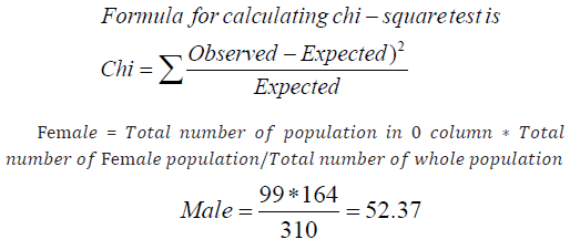
This is another chart which gives the representation of disease patients in male and female the blue one is the male and the green is the female the test which is called chi test is performed to check the null hypothesis HO is proposed Null hypothesis claims that disease does not interact with the gender of the population if the hypothesis is refuted that disease has some association with the gender of the population (Graph 2). The overall amount of men in Table is 208, and the female population is 99. The columns range from no heart attack to seriously dangerous heart disease is 0,1,2,3,4 and their cumulative values are approximately 164, 56, 37.5, 37.5 and 15. It measures the estimated number of patients who are sick. One explanation as to how the predicted number for the 0 column is extracted is as follows:
Graph 2

There are 5 columns and 2 rows in the table which are the female and male (Table 5). The degree of freedom for this degree is (R-1) * (C-1) where C and R are columns and rows accordingly the extent of equality then is 4 the chi-square value of test achieved is 23.35, which is higher than the distribution table value of 9.488 of chi-square. the hypothesis is thus denied therefore with 95% certainty it can be claimed that the disease has some association with gender this results as seen in figure that female population is less vulnerable than the male population of the heart disease (Graph 3). The above figure demonstrates the values of the no heart disease to heart disease in male and female Cp varies from 0 to 3 indicating the chest pain type (0: atypical angina, 1: normal angina, 2: non-angina, 3: Asymptomatic). It can be found in this data collection that asymptomatic chest pain is more likely to have heart disease in the population diagnosed with chest pain type 4
Table 5: Planned sex-based number of diseased patients.

Graph 3

Result and Implementation
This chapter discusses the conclusions of the Cleveland dataset review and provides a comparative examination of algorithms. The data collection was used on various machine learning algorithms, also known models, after both pre-processing, exploratory analysis. and descriptive
Pre-Processing of Data
As previously discussed, one of the most critical phases is data pre-processing to achieve the best from the data collection. In Machine Learning, it is really crucial. We would concentrate on data recovery, the handling of lost values, data transformation and discretization of data.
In the Scikit-learn machine learning library, named Label Encoder and One Hot Encoder, two classes are found. Basically, Label Encoder translates categorical values into numbers that are ordinary in nature. There are categorical variables such as Cp, chest pain type, defined as 1,2,3 and 4, in the data set used for this analysis. here is no ordinary connection between 1,2,3 and 4, but when added explicitly to machine learning algorithms, it provides incorrect results. Thus, One Hot encoder is used to encode values of the chest pain form into binary values, addressing the problem of multiple sources of evidence. The dependent variable or attribute to be expected is multi-class in this data set. This varies from 0 to 4. But the multiclass dependent variable is transformed into a binary class for this analysis.
Experimentation
with the Cleveland dataset, numerous machine learning and deep learning models were tested. Originally, a data set is modelled in this analysis without feature selection and the findings were achieved and only with feature extracted from SBS were modelled in the second process. Techniques such as k-fold cross validation and parameter tuning were used in both studies. K-fold cross validation is a tool used for a dataset to prevent model over-fitting and under-fitting, and parameter tuning is a method that helps to find the right parameters for the model employed.
Training
A training set is the knowledge component of which the model is trained. 70 percent of the data are used for instruction in this analysis. In particular, 60 to 70 percent of the training dataset is used in machine learning groups, although it differs widely based on the need and intent of the study. The consistency of training is also high in data training, which means the model displays a high degree of consistency in the training collection, but when measured against the test set, the productivity is weak, So, k-fold cross validation has been used to prevent output errors. For e.g., in k-fold cross validation, 10-fold cross validation, training set is divided into 10 parts but from every 10 component, test and training set is described and model is used and the outcome of all ten parts is summed, which helps to reduce the data over fitting or under the fitting.
Testing
A testing set is the component of the knowledge where model is evaluated, also the dependent data variable. 30 percent of the information was used for testing in this study. based on the model used, it will do better or worse when cross-validated data is checked. Therefore, a method called parameter tuning has been used to ensure that any model operates optimally. The Scikit-learn library includes the Grid Search CV class that performs the tuning of parameters.
Results
The goal of the whole project was to evaluate which algorithm better identifies diseases. This segment contains all the outcomes of the analysis and presents the top performer based on different performance metrics. Firstly, efficiency was obtained in the training set by using 10-fold cross validation. Lastly, efficiency was attained only by using the standard without tuning any parameters, tuning third parameters and calibrating the fourth standard. The tables below present the performance (Table 6). Decision Tree provided the best performance in the 10-fold cross validation, characterised by Random Forest, KNN, SVM, Naïve Bayes and Logistic Regression referring to Table 7. The Table 7 shows the appraisal of algorithms with the extreme boost tuning are as follow Extreme gradient boost has achieved the highest efficiency, followed by the others KNN did better in the test set than in the training set but KNN ROC is relatively high than SVM its means that the SVM accuracy is not exactly correct the classifier is overfitted In Table 8, the row of Naïve Bayes is Zero since parameter tuning is not required, there are no parameters to be tuned in Naïve Bayes. Thus, for performance comparison, the results from Table 9 were taken. KNN and logistic regression in training and decision tree in testing efficiency goes down after parameter tuning. After parameter tuning, XGB is the best performer, followed by Naïve Bayes and Random Forest in training and logistic regression followed by Naïve Bayes, KNN and random forest in testing.
Table 6: Assessment of training set of algorithms using k folds.

Table 7: Appraisal of algorithms with the extreme boost tuning.

Table 8: Algorithm evaluation in train range, parameter optimised by calibration.

Table 9: Algorithm evaluation in test range, parameter optimised by calibration.

Deep Learning Algorithm
The algorithm used in this research is the Artificial Neural Networks (ANN). the ANN metrics for performance are shows as below (Table 10). The hidden layer used in ANN were three as shown in the table uses the ‘adam’ algorithm as an optimizer as well. The parameter ANN was calibrated to the machine learning library of keras CNN is originally worked with 2 convolution layers of 91 attribute maps and 4 layers of 1024 secret units, each totally connected. For various numbers of convolutional layers, the output of the device is often evaluated. After, with the same number of function maps, we raise the convolutional layers from 2 to 5 to notice the results of the convolutional sheet. Notice that in completely linked layers, no modification is made. For 3 coevolutionary layers, the best efficiency, i.e. 96% precision, is obtained (Table 11).
Table 10: for Artificial Neural Network Assessment.

Table 11: Comparative analysis of results with a different number of convolutional layers.

The Performance Comparison
Different algorithms worked better depending on the situation from all the tables above, whether cross validation, grid search, calibration, and feature selection are used or not. Based on the case, each algorithm has its innate potential to outperform other algorithms. For example, with a large number of datasets, logistic regression performs much better than when knowledge is small, whereas decision tree performs better with a smaller number of data sets. After applying exa boosting the data that was not featured, algorithm efficiency increased. Chosen though algorithms worked better without boosting in the not chosen function Data. After boosting the results, the performance of algorithms improved. Selected functionality while the efficiency of the algorithm decreased after boosting the selected function Data. This highlights the need for the data to be chosen before feature selection. Boosting compliance. Output metrics after features for dataset comparison Collection, tuning and calibration of parameters are used since this is the normal procedure for Assessing algorithms. Performance measures of classifiers are contained in Table, so that the region under the ROC curve of the test should be used as a parameter to calculate the discriminative potential of the test, i.e. how successful the test is in a given clinical scenario. Tests are usually classified based on the area under the ROC curve. The closer the upper left corner of a ROC curve, the more effective the test is. Averaged value of SVM, Naives Bayes and extreme boost are 88,88,87 respectively which shows that SVM and Naïve Bayes performs an average.
When it comes to deep learning ANN has scored not that so much good classification accuracy as the Table ANN classifier with an overall value of 0.72 regardless of the contrast of all the machine learning algorithm with ANN. But when implemented in a medical environment, ANN has a challenge, since there is little space for the analysis of the data. ANN functions like a black box, but it cannot be totally believed until learning how it operates. Well CNN has scored the best accuracy ratio with an overall number of 0.91 compared to ANN and all the machine learning algorithm which scored lower when implemented as a clinical trial the performance for 3 convolutional layers gives the best result with higher efficiency
The aim of the project was to equate the algorithms using machine learning and deep learning with various performance metrics. All the data are pre-processed and used for the test estimation. In one case, each algorithm worked better and worse in another. The probable models to work better in the dataset used in this analysis are SVC, CNN and Naïve Bayes. There are also consequences for being able to reliably detect heart failure through machine learning. It is possible to produce various instruments that track the events associated with the heart and diagnose the disorder. Where heart disease specialists are not present, these instruments can prove to be beneficial. Machine learning can also be used to detect heart failure with further testing before human doctors can do so. This one of the project’s greatest successes was that the project came to better understand algorithms. The algorithms behaved differently when evaluated in various conditions, which made me understand the operating process of the algorithm. With machine learning and deep learning this work will be the first learning step in the diagnosis of heart disease and can be further applied for future study. There are many drawbacks to this research, namely the author’s knowledge base, secondly, the instruments used for this study, such as with the computer’s computing power and, thirdly, the time limit available for the study. This style of research requires state-of-the-art infrastructure and experience in the related fields.


