Identification of Melanoma Cancer Using Feature Extraction from Medical Image Textures by Artificial Intelligence Volume 58- Issue 3

Marcos A M Almeida*

• Department of Electronics and Systems, Technology Center, Federal University of Pernambuco, Recife-PE 50670-901, Brazil

Received: August 14, 2024; Published: August 27, 2024

*Corresponding author: Marcos A M Almeida, Department of Electronics and Systems, Technology Center, Federal University of Pernambuco, Recife-PE 50670-901, Brazil

DOI: 10.26717/BJSTR.2024.58.009148

Abstract PDF

The objective of this study was to identify the best attributes for diagnosing melanoma, based on texture data from medical skin images using the primary color channels: red, green and blue. The best attributes are part of Haralick’s second-order stat set. Classification models were then used to obtain early diagnosis of randomly chosen medical images on a test basis. The research presented Histogram Gradient Boosting as the best classifier for the red and green channels, with an accuracy of 99.00% and AUC of 99.98% for the red channel, an accuracy of 88.00% and AUC of 93.35% for the green channel. The blue channel data was best classified by the Random Forest algorithm with an accuracy of 85.00% and an AUC of 92.82%.

Keywords: Artificial Intelligence; Machine Learning; Digital Image Processing; Image Classification; Image Diagnosis.

Abbreviations: AUC: Area Under Curve; CNN: Convolutional Neural Network; GLCM: Gray Level Co-occurrence Matrix; KNN: KNearest Neighbors; ROI: Region of Interest; ROC: Receiver Operating Characteristics; SVM: Support Vector Machine; XGBoost: eXtreme Gradient Boosting

Image classification using machine learning/artificial intelligence techniques and algorithms plays an important role in the diagnosis of early diseases. This is because specialists’ human eyes cannot detect small differences in pixel intensities that represent texture variations in high-resolution medical images. Through learning techniques, with the extraction of characteristics from images, algorithms through training and testing, it is possible to classify these images, using the most relevant attributes. Julesz proved that certain discriminations of locally evaluated texture pairs were only possible with the calculation of second and third order statistics. “So, if iso-second-order texture pairs yield effortless discrimination, this must be the result of local features, to be called textons” [1-4]. Therefore, this research includes attributes such as feature extractors from sampled images with the calculation of the GLCM matrix for the red, green and blue channels. Computer procedures and advancements in machine learning not only aid the dermatologists in early detection of melanoma but also avoid heavy expenses of melanoma detection and unnecessary biopsies. Novel automatic melanoma detection systems save a lot of time, money, and effort. Machine learning has proven to provide melanoma classification with improved and higher accuracies [5]. Figure 1 shows medical images of melanoma and nevus with sixteen sample matrices for each of them. The histograms of the sixteen image samples of a melanoma randomly chosen from the database are shown in Figure 2. In each of the sixteen regions of interest, histograms were calculated for a nevus image, as shown in Figure 3.

Figure 1

Figure 2

Figure 3

According to Julesz [1-4] to better extract texture features for image classification purposes, it is necessary to calculate first and second order statistics: First-order statistics measure the likelihood of observing a gray value at a randomly-chosen location in the image. First-order statistics can be computed from the histogram of pixel intensities in the image. These depend only on individual pixel values and not on the interaction or co-occurrence of neighboring pixel values. The average intensity in an image is an example of the first-order statistic. Second-order statistics are defined as the likelihood of observing a pair of gray values occurring at the endpoints of a dipole (or needle) of random length placed in the image at a random location and orientation. These are properties of pairs of pixel values [6].

The extraction of image features is obtained from the histogram of intensities as well as the features that make up the co-occurrence matrix (GLCM). Thus, an image can be represented by a function f(x, y) of two discrete variables x and y, with , x = 0, 1,…, N − 1 and y = 0, 1,…, M − 1, a discrete function f (x, y ) can take values for i = 0, 1,…, L − 1, where L is the maximum intensity level of red, green, blue or grayscale colors. The intensity level histogram is a function that shows (for each intensity level) the number of pixels in the entire image, which have this intensity:

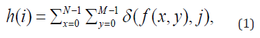
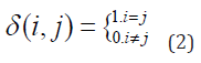
where (i, j) is the Kronecker delta function.

For each region of interest, p (i) can be calculated, which is the normalized probability, shown in Figure 1.

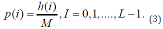
Table 1 shows the first-order statistics, while Figure 4 shows the neighborhood of the pixels to be analyzed.

Table 1: Attributes that belong to first-order statistics.

Figure 4

The gradient of an image is a measure of the spatial variations of color levels in the image. The gradient can be negative or positive, depending on whether the color level varies from the darkest to the lightest tone or vice versa. For each pixel within the ROI-defined region of interest or within the sliding mask, as illustrated in Figure 1, an absolute value of the image gradient is calculated, according to Equation (8):

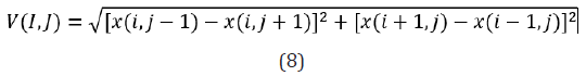
Table 2: Attributes that belong to second-order statistics.

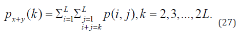
A set of scalar quantities to summarize the information contained in a Gray Level Co-occurrence Matrix – GLCM was proposed by Haralick, which can be defined as a second-order histogram. It is a square matrix formed by elements that indicate the probability of occurrence of a pair of pixels with intensities that depend on the distance from angle θ. This takes into account the frequency of a pixel with the intensity of the gray level. Value i occurs in a specific spatial relationship to a pixel with value j. Each element (i, j) in the GLCM is calculated by summing the number of times the pixel with value i occurred in the specified spatial relationship to a pixel with value j in the input image [7]. Equations 13 to 20 constitute the set of second-order statistics. In this research, not the shades of gray were considered, but applied to the red, green and blue channels.

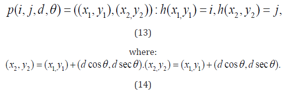
In this research, the distances considered were d = 1, with angles θ = 0°, 90°, 180° and 270°. Pixels located on diagonals were not considered. GLCM expresses the texture feature according to the calculation of the conditional probability of the pixel pair of gray intensities for different spatial positions.

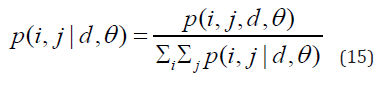
Table 3: Attributes that belong to second-order statistics.

Where

In academic medical literature, instances are designated as positive, indicating the existence of the disease, and negative, indicating the absence of the disease; thus, four possibilities arise when medical images are submitted to the classifiers: The metrics that were considered to evaluate the classifiers for these were: Table 4. Performance metrics for classifiers

Table 4: Performance metrics for classifiers.

The study database consisted of 64 images in bitmap format, randomly selected from the ISIC database, 32 images of melanoma and 32 images of nevus. 16 samples were extracted from each image, making a total of 1024 samples. Each sample consists of an 8 x 8 pixel region of interest. In each roi, 53 attributes were calculated for feature extraction, composing first and second order statistical information, including a co-occurrence matrix, based on Haralick’s texture characteristics. This was calculated for the red, green and blue color channels, according to the process shown in the block diagram in Figure 5. The total samples were divided into the training database in the proportion of 75%, 768 samples, and 25% of the samples, destined for testing, 256 samples. The Machine learning classification models applied to data referring to medical images from the red, green and blue channels, were:

1) Logistic Regression.
2) Random Forest.
3) Histogram Gradient Boosting.
4) Gradient Boosting.
5) Gaussian Naive Bayes.
6) Ada Boosting.

After validating the best model that fits the data referring to the melanoma and nevus image samples, the seven best attributes that contribute to the model were identified, in the classification of images, and consequently in the decision whether melanoma or nevus, using the shape function value from the Python environment library.

After the operational implementation described in the block diagram in Figure 5, the results were obtained for each of the red, green and blue color channels.

Figure 5

The model that best fitted the red channel image data was Histogram Gradient Boosting, with an accuracy of 99.00% and an AUC curve area of 99.98%, as shown in the data in Table 5. Figure 6 shows the second and third best models, in the red channel, according to the AUC curve, they are Gradient Boosting and Random forest, respectively. A suitable overall measure for the curve is the area under the curve -AUC. A good classifier is one whose AUC is close to 1. The ten best attributes in feature extraction using the red channel of the studied melanoma and nevus image samples are shown in Figure 7, using the shape value function. The sum of the average intensities between neighboring pixels (Eq. 21) are among the five best attributes.

Table 5: Metrics associated with the performance of the best data classifier of images from the red channel – HistGradientBoosting.

Figure 6

Figure 7

Similar to the red channel, the Histogram Gradient Boosting classifier was the best, among those studied, for classifying melanoma and nevus images in the green channel, with an accuracy of 88.00% and an AUC of 93.35%. There was also greater accuracy in identifying images with melanoma - 90.00%, than identifying nevus images - 86.00%, according to data shown in Table 6. In addition to the Histogram Gradient Boosting classifier, two others performed well, according to AUC values, the random Forest with an AUC of 92.31% and the Gradient Boosting with an AUC of 91.43%, as shown in Figure 8, through the ROC curve. Figure 9 shows the ten main attributes of feature extraction are the sum of the average intensities between neighboring pixels (Eq. 21), among the five main attributes that best contribute to the classification model. The others are the contrast (Eq. 17), the variance difference (Eq. 25) and the correlation (Eq. 18) between pixels, according to the shape value method Table 6.

Table 6: Metrics associated with the performance of the best data classifier of images from the green channel – HistGradient Boosting Classifier.

Figure 8

Figure 9

The best classifier for the image data presented in the blue channel was Random Forest with an accuracy of 85.00% and an AUC of 92.82%. The ROC curve shown in Figure 10, for the images filtered in the blue channel, assigns the second best classifier as Histogram Gradient Boosting and the third as Gradient Boosting, with AUC of 91.28% and 90.14%, respectively.Several attributes make up the first ten elements that best contribute to the model of this classifier that operated in the blue channel: RandomForest. They are in order of intensity and importance: Figure 11 Difference variance (Eq. 25), difference entropy (Eq. 26), Average intensity of the blue color (Eq. 4), sum of average intensity (Eq. 21), correlation (Eq. 18), always with respect to neighboring pixels.

Table 7:

Figure 10

Figure 11

Mehwish Dildar, et al. [8], using a comparative analysis of skin cancer detection using SVM-trained CNN, extracted features, with a median filter for noise removal, obtained an accuracy of 93.75%. The method proposed by Mohammadreza Hajiarbabi, using the MobileNetV2 [9] network, the CNN with 53 layers, using a set of skin cancer images from the ISIC 2020 database, achieved an accuracy of 94.4%. Extremely Randomized Trees classifier, commonly known as “Extra Trees Classifier” represents a version of random forest which obtained the best performing method, with an accuracy of 97.00%, in the study carried out by Revanth Chandragiri Revanth Chandragiri, et al. [10]. Using Fine Neural Networks for skin disease classification solution, Lee, et al. [11] achieved an accuracy of 89.90% and 78.50% on the validation set and test set, respectively. Rahul, et al. [12] used several CNN-type models with different databases and achieved accuracies ranging from 85.65% to 97.01% Models such as SVM, KNN, XGBoost, Standard Cascade Forest were used by Safa Gasmi, et al. [13], where the best accuracy values were found in the Proposed Modified Standard Cascade Forest model with a value of 76.26%. Asmae Ennaji, et al. [14] used color, geometric shape, texture, and fusion of all tumor features as inputs for image classification. The support vector machine model was run to identify melanoma diagnosis. Of the six strategies used, the one with the best response was the one that took into account voting software, achieving an accuracy of 99.00%.

Ansari [15] using dermoscopic images of skin cancer subjected it to different preprocessing strategies using filters, and later calculating GLCM parameters, selected specific highlights in the image which were then used to help establish the SVM classifier. Table 6 The classification determined whether the image was of a cancerous or non-cancerous tissue. The accuracy of the proposed framework is 95.00%. Anis Mezghani, et al. [16], presented in this study a model that represents a significant advance in the field of skin cancer detection by employing a combination of Convolution Neural Networks and Support Vector Machines, using images with data augmentation, for the accurate categorization of skin lesions into benign and malignant forms, reaching accuracy values of 98.71%. It was observed in this study that the best classifier was the Histogram Gradient Boosting, when applied to image sample data from the red channel, produced the best feature extraction, whose response was an AUC of 99.98% and an accuracy of 99.00%. It was also the best classifier for extracting features from the green channel, being the second best in the blue channel. The “SumAvarege” attribute, derived from the Co-occurrence Matrix calculations, when applied to neighboring pixels in the image samples, was the most relevant attribute, among the 53 calculated in this study, and which contributed significantly to the Histogram Gradient Boosting model, so that it reached excellent levels for AUC and accuracy values, when the images were submitted to the red channel (positions 1,2, 4 and 5).

The “SumAverage” attribute also appears as the most important for the Histogram Gradient Boosting model, with a response of an AUC of 93.35% and an accuracy of 88%, when applied to neighboring pixels in image samples submitted to the green channel (positions 1, 2 and 6). The results obtained in this research were better than the previous results [17-18], Table 7 where the models were modified as well as the way of identifying the best attributes.

Acknowledgments

Authors may acknowledge those individuals who provided help during the research and preparation of the manuscript. This section is not added if the author does not have anyone to acknowledge.

Author contributions

Not applicable.

Conflicts of Interest

The authors declare that they have no conflicts of interest.

Ethical Approval

Not applicable.

Consent to Publication

Not applicable.

Availability of Data and Materials

Not applicable.

Funding

Not applicable.

1. Julesz B (1981) Nonlinear and Cooperative Processes in Texture Perception, In Theoretical Approaches in Neurobiology, MIT Press Cambridge MA P. 93-108.
2. Julesz B, (1980) Spatial nonlinearities in the instantaneous perception of textures with identical power spectra. Philos Trans R Soc London B 290: 83-94.
3. Julesz B (1981) Textons, the Elements of Texture Perception, and Their Interactions. Nature 290: 91-97.
4. Julesz B (1981) A Theory of Preattentive Texture Discrimination Based on First-Order Statistics of Textons. Biological Cybernetics 41: 131-138.
5. Arslan Javaid, Muhammad Sadiq, Faraz Akram (2021) Skin Cancer Classification Using Image Processing and Machine Learning. Proceedings of 2021. 18th International Bhurban Conference on Applied Sciences & Technology (IBCAST) Islamabad Pakistan 12-16 January PP. 439-444.
6. Tuceryan M, Jain AK (1998) Texture Analysis. The Handbook of Pattern Recognition and Computer Vision (2^nd,). 207-248.
7. Robert M Haralick, K Shanmugam, ItsHak Dinstein (1973) Textural Features for Image Classification. IEEE Transactions on Systems Man and Cybernetics SMC-3 6: 610-621.
8. Mehwish Dildar, Shumaila Akram, Muhammad Irfan, Hikmat Ullah Khan, Muhammad Ramzan, et al. (2021) Skin Cancer Detection: A Review Using Deep Learning Techniques. Int J Environ Res Public Health MDPI 18(10): 5479.
9. Mohammadreza Hajiarbabi (2023) Skin Cancer Detection using Multi-scale Deep Learning and Transfer Learning. Journal of Medical Artificial Intelligence 6: 23-67.
10. Revanth Chandragiri, Koti Satya Prabhudev Badarla, Kavitha Modepalli, Dwarampudi Balaji Reddy, Anwar Hussain Syed, et al. (2024) A Systematic Review on Machine Learning Techniques used for Early Detection of Skin Cancer. 13 th IEEE International Conference on Communication Systems and Network Technologies Pp. 862-867.
11. Yeong Chan Lee, Sang Hyuk Jung, Hong Hee Won (2018) WonDerM: Skin Lesion Classification with Fine-tuned Neural Networks. In ISIC 2018 Lesion Analysis Towards Melanoma Detection Cornell University Ithaca NY USA P. 1-4.
12. Rahul, Rakesh Kumar, Meenu Gupta, Ahmed J Obaid (2024) A Deep Learning Based Critical of Skin Lesion Classification. 2024 International Conference on Advances in Modern Age Technologies for Health and Engineering Science (AMATHE) 01-05.
13. Safa Gasmi, Akila Djebbar, Hayet Farida Merouani, Hanene Djedi (2024) An Innovative CBR-Enhanced Approach for Skin Cancer Classification using Cascade Forest Model and Convolutional Neural Network with Attention Mechanism. EAI Endorsed Transactions on Pervasive Health and Technology 10: 01-14.
14. Asmae Ennaji, My Abdelouahed Sabri, Abdellah Aarab (2024) Ensemble learning with weighted voting classifier for melanoma diagnosis. Multimedia Tools and Applications. Springer P. 01-17.
15. Uzma Bano Ansari (2017) Skin Cancer Detection Using Image Processing. Int Res J Eng Technol 4:2875-2881.
16. Anis Mezghani, Sonia Slimen, Monji Kherallah (2024) Skin Lesions Diagnosis Using ML and DL Classification Models. International Journal of Computer Information Systems and Industrial Management Applications 16: 117-130.
17. Marcos AM Almeida, Iury AX Santos (2021) Analysis and Classification of Skin Spot Images by Extraction of Texture Attributes for Identification of Melanoma. Biomed J Sci & Tech Res 35(2): 27505-27514.
18. Marcos AM Almeida, Iury AX Santos (2020) Classification Models for Skin Tumor Detection Using Texture Analysis in Medical Images. Journal of Imaging 6(51): 01-15