Skull-Face Matching Based on Principal Component Distance of Anatomical Features Volume 57- Issue 3

Gong Huangkai¹, Wu Henderson¹, Wan Xinyi¹, Gu Zhongya¹, Ma Zhongbin² and Ji Dafeng¹*

• ¹Medical College of Nantong University, China
• ²Nantong Hospital of Traditional Chinese Medicine, Nantong, China

Received: July 01, 2024; Published: July 09, 2024

*Corresponding author: Ji Dafeng, Medical College of Nantong University, China

DOI: 10.26717/BJSTR.2024.57.009008

Abstract PDF

ABSTRACT

Objective: To investigate the value of principal component distance of anatomical features in cranial-face matching.

Methods: Human head CT data were 50 cases, including 25 males and 25 females. Each skull and facial tissue were reconstructed and stored in the skull and head database, respectively. Six anatomical features in the skull were determined, coordinate points were recorded, and the covariance and principal component coefficients of coordinate points were calculated. The mean and standard deviation of the principal components are calculated by finding the coordinates of the markers, and the mean and the standard deviation are saved in order as a database as the digital mapping of skull-face. The Euclidean distance is compared between the skull principal component coefficient and the principal component coefficient of the database skull model to be matched, and the face model mapped by the minimum distance is taken as the result of the skull face simulation. Rebel the 40 skull anatomical feature points in the model library and match the skull model in the database to verify the reliability and robustness of the data algorithm.

Results: The correct number of matches in the database was 37 (92.5%).

Conclusion: The principal component distance based on anatomical features can effectively match the facial data corresponding to the skull.

Keywords: Anatomical Characteristics; Principal Component Coefficient; Euclidean Distance; Face Restoration; Database

Introduction

Face restoration technology based on skull has always been a research hotspot in archaeology and forensic medicine [1]. The traditional recovery technology obtains human head data through CT scan, and after reconstruction, the skull model is obtained through 3D printing or gypsum model, and the soft tissue modeling is performed on the model to obtain the effect of facial recovery. This kind of recovery requires high time cost, large material demand, low recovery effect compliance rate, and no digital storage or modification. In view of the above deficiencies, this study plans to establish a digital skull-face database, combined with the spatial distance between the principal components of the skull, so as to map the facial features of the skull.

Data

General Information

Human head CT data for 50 cases, including 25 males and 25 females; scan range: roof to full jaw; scan voltage: 120kV; resolution: 0.49mm×0.49mm×0.5mm; scanning machine: Philips; Workstation: HOST-32348. DICOM (Digital Imaging and Communications in Medicine) Data were provided by the Imaging Center of Nantong Hospital of Traditional Chinese Medicine.

Software platform

Image processing platform: 3DSlicer 5.6.1 (www.slicer. Og); Data processing and programming: MATLAB R2016a (Mathworks corp., USA).

Methods

Based on the CT data of the skull in the study, the study was located to six anatomical feature points and matched the three closest skull in the database and their faces through the principal component coefficient distance of the feature points. The specific experimental flow is shown in the figure below.

Location of the Anatomical Markers

The data was volume rendered (Volume Rendering) in 3DSlicer, using Create new Point List to create a set of mark points, respectively in the left cheekbone, the nasal root, the end of the nasal bone, the right cheekbone, the maxillary middle incisor, and the mandibular mental process, to create a set of 6mark points (Figure 1). After positioning, the coordinates were copied in the Markups module and imported into Excel for numbering.

Model Reconstruction and Export

The skull and face were reconstructed by the threshold, cut off the excess, open the Surface Toolbox, select the model, and the optimization rate was adjusted to 0.9 in the Decimate module, and the model was optimized to reduce the number of vertices and polygons and increase the extraction efficiency. The optimized skull model and face model are exported as stl (stereolithography) to form the model database. The database includes the skull model library and face model library, where the corresponding skull has the same number as the face model.

Digitization of Anatomical Features and the Formation of a Feature Database

The coordinates in 2.1 were imported into MATLAB to calculate the covariance matrix (Formula 1), and the principal component coefficient was calculated by using the covariance matrix.

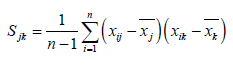
Where n is the number of feature points, n =6, p is the number of feature dimensions, p =3, representing the X axis coordinate, Y axis and Z axis coordinate, x_ij, x_ik, x_j, x_k Represents the coordinate values of the corresponding axis, and the mean of the corresponding axis coordinates, Sjk is the covariance matrix of the coordinate matrix. The covariance matrix eigenvalue and the eigenvector, and the first principal component coefficient under the maximum eigenvalue. The MATLAB command used in the above procedure is:

S = cov (Coordinates); % to find the covariance matrix of the coordinate matrix

[C, ~, lam] =pcacov (S); % Find the principal component coefficient coeff and the variance contribution lam of the covariance matrix.

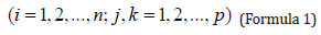
This gives a symmetric square array of 3×3. Save the square matrix in sequence as a feature database. The cumulative contribution of principal components was calculated from the variance contribution, and the cumulative contribution of the first two principal components was> 90%. The first and second principal components of the marker points were found using Formula 2 and recorded into the digital feature library.

Where n is the number of samples, i is the main component serial number, Y_ni is the sample principal components, F_n is the point coordinates for the sample, C_i is primary component coefficient.

Digital Feature Distance Calculation

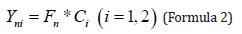
According to the cumulative contribution rate of principal components in 2.3, and the mean value and standard deviation of the first principal component coefficient and the second principal component are taken as the digital features, and the Euclidean distance (formula 3) between the matching marker and the digital feature library is obtained as the evaluation index of skull similarity.

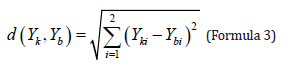
Y_k is the principal component numerical features of the skull to be matched, Y_b is the numerical feature of the principal components in the principal component coefficient library. The smallest of these 3 distances were selected as the reference model output (Formula 4).

Where Y_k is the principal component coefficient of the skull to be matched, F_i is the minimum face in 3 matched faces.

Model Rotation Validation

By rotating the angles of existing models X, Y and Z axis, calculate the digital features at different angles and then compare their similarity.

Program Testing and Packaging

Design the graphical user interface, define appropriate buttons, graphical display axes, options and other components (Figure 2), and embed coordinates records in the software.

Regeneration Misjudgment Rate

Using the 40 skull models in the database, we re-labeled the feature points, and then conducted the matching accuracy test to calculate the matching success rate. Where the minimum, mean and maximum Euclidean distance are determined more than 2 times, the same number is recorded as the matching result. The backward misrepresentation rate is calculated by Formula 5.

among n* Is the number of misjudgment, n is the total number of cases, here n =40, E is the backward misjudgment rate.

Results

Principle Component Coefficient of Anatomical Features

Model 4 in the selected database for matching validation and Figure 3 shows the coordinates of the selected data points. Table 1 shows the database skull original feature coordinates and principal component coefficients and the relabeled feature coordinates and principal component coefficients. As can be seen from Table 1, the coordinates of the feature points are changed, but the principal component coefficients are less different. As can be seen from Table 2, the digital features of the marked points of the same model vary very little under different angles.

Validation Results

According to the first and second principal component characteristics in Table 2, the corresponding minimum 3 distances in all samples are selected, and the corresponding face and skull models are extracted through the mapping of the principal component digital feature library and displayed. In this case, the no. 4 skull model is verified, and Figure 4 shows the matching results. As Figure 3 illustrated, the similarity and distance order are 15 (0.00315), 12 (0.04292), 4 (0.05555), 4 (0.08984), 11 (0.1.11736), 15 (0.12741), and the maximum matching order is 4(0.12413), 11 (0.17435), 10 (0.23217). The skull model is considered to match successfully.

According to Formula 4,37 cases were successfully matched to the original skull, with a matching success rate of 92.5%.

Discussion

The restoration of skull appearance is of great significance to the attributes of archaeological, forensic and biological species. In the two-dimensional images, the defective face is currently used to restore the face [2], A fuzzy face restoration based on the da Vinci platform [3]. However, there have been few studies on three-dimensional face restoration, due to the large difference in soft tissue and the unknown relationship between skull-soft tissue. Since the skull anatomical features play an important role in CT-MRI image fusion [4-6], The skull is also the foundation of the soft tissue of the head and face. Therefore, using the anatomical features of the skull. The obvious anatomical features of the skull include anterior and posterior diameter, transverse diameter, agittal angle, occipital tuberosity (convex) and the height of cribriform crest [7] Etc., these features have an important role in intracranial image fusion, but cannot be used for craniofacial data fusion or matching. In the application of body surface structure, the localization error of anatomical features based on CT is smaller than that of that based on MRI, and the applied features include 8 structures, including eyebrow center, ear wheel and occipital protrusion [8]. According to Zhou et al., the features based on the key points of expression have a higher recognition accuracy and the feature data are more concentrated [9], The corresponding computational amount also showed significant decreases, indicating that facial expressions have obvious correlation with anatomical features, but these temporary facial features [10], And does not serve as a key point for cranial-plane matching.

Therefore, the anatomical features consistent with the personalized face must be found to be applied to the cranial-plane matching data. The zygoma can be used as a three-dimensional evaluation feature of facial soft tissue defects as described by Elena et al [11], And the zygomatic bone is also the widest part of the face, as the maximum variance of the feature point on the coronal axis. The Angle between the frontal and nasal angles, the upper end of the nasal bone, and the connection at the end of the nasal bone, varies greatly in different races or among different individuals [12], The frontal nose angle can be regarded as the maximum variance of the feature point in the sagittal axis and can be used as a cranial-cranial match. The convex shape of chin lung is divided into round, square and pointed, and there are great differences in different races or different periods [13], Thus it can also act as markers of cranial-cranial matching. Among the differences in cranial structure, the genetic influence rate of the dental arch of permanent teeth was as high as 72.92% [14], Therefore, the nasal root-chin bulge distance can be regarded as the maximum variance of the feature point on the vertical axis and also as a sign of cranial-cranial matching. The matrix principal component difference is mainly based on its eigenvalues and eigenvector, which represents the main direction of point cloud distribution in 3 D space and is the calculation of principal component coefficients. Based on the anatomical features described above, the basic structures of interskull matching include zygomatic, nasal root, nasal bridge, dental arch, and mental bulge of the mandible. As a technology of dimension reduction analysis, principal component analysis can reduce the complex face point cloud [15], Thus the principal component distance is calculated and used as a feature similarity [16].

The advantage of PCA coefficient is not affected by original coordinate point scaling, rotation and translation. PCA is also a linear fit to multivariate data, so too many dimensions are prone to overfitting. In the pre-experiment of this study, the 9 feature points showed an obvious overfitting state. Based on the above basis, this study uses the six craniofacial anatomical features of the skull CT sequence to obtain the principal component coefficient and match the most similar facial skull through the calculation of Euclidean distance, combining the existing cranial surface data, so as to map the most consistent facial structure. To analyze the reliability of matches from the backward misjudgment of known model libraries, as shown in Table 1, the obtained principal component coefficient is very close in different feature coordinates. Further, by solving the principal components, the mean and standard deviation of the first principal component and the second principal component are obtained as the digital features of the model. Combined with the Euclidean distance, the similarity between the matching model and the model in the database can be evaluated. As visible from Figure 4, the matching model matches the model to be tested. The accuracy reached 92.5% by the reciprocal test of data from 40 cases (Figure 5).

Conclusion

The corresponding faces could be matched to the skull based on the Euclidean distance of principle component coefficient.

Support Fund

Nantong Social Livelihood Project-Development and Application of Medical Imaging Positioning System in Minimally Invasive Orthopedics (MS12021089).

References

1. Enghong D (2012) Research on the realistic treatment technology of skull recovery. Chang'an University.
2. Tingting S, Na W (2019) Face restoration algorithm based on image block similarity and completion generation. Science, Technology and Engineering 19(13): 171-176.
3. Xuefeng W, Jianming L (2013) Implementation of a fuzzy face restoration algorithm on the Da Vinci platform. TV Technology 37(7): 9-12.
4. Tengfei X (2012) 3D reconstruction of CT-MRI fusion images in navigation 3 D visualization of sinus-skull base surgery. Chinese PLA Medical College.
5. Rong Y, Qingxiang L, Chi M, Xin Peng, Yang Wang, et al. (2019) Multimodal imaging fusion technology and the diagnosis and treatment of tumors in the skull base-inferior temporal region. Journal of Peking University (Medical edition) 5(1): 53-58.
6. Zhiqiang L, Xiaoshu L, Jiyong X (2022) Application of DSlicer multimodal image fusion in meningioma surgery. Chinese Journal of Clinical Neurosurgery 26(10): 758-760.
7. Li G, Xiaohua Z, Baojun X (2004) Correlation analysis between skull morphology and skull anatomy in China. Journal of Wuhan University 25(3): 292-294.
8. Dafeng J, Zhongbin M (2019) Bimodal fusion of human head based on surface anatomical features. Journal of Anatomy 50(5): 638-644.
9. Zhou Y, Liang Y, Tan P (2023) Design of an intelligent laboratory facial recognition system based on expression keypoint extraction. IEEE Access 11: 129805-129817.
10. Hong K (2022) Facial expression recognition based on anatomaly feature. Optical Review 29(3): 178-187.
11. Elena GO, Federica M, Sandro M, Alberto Ferrando, Enrico Vezzetti, et al. (2021) Three-Dimensional Evaluation of Soft Tissue Malar Modifications after Zygomatic Valgization Osteotomy via Geometrical Descriptors. J Personalized Med 11(3): 205.
12. Wei T, Yaqiong G, Xianlu W (2021) Clinical results and experience of integrated surgery of autologous costal cartilage nose. Anhui Medicine 42(10): 1155-1158.
13. Shuping D, Haijun L (2014) Variation of modern mandibular chin shape and comparison with fossil humans. Journal of Anatomy 45(6): 847-850.
14. Jing L, Jinghui Z, Yichao Q (2015) Inheritance of crown and arch in adolescents. Chinese and Foreign Medical Care (9): 15-17.
15. Sharma R, Patterh MS (2015) A new hybrid approach using PCA for pose invariant face recognition. Wireless Personal Communications 86(3): 1561-1571.
16. Chung ST, Seongwon C Robust (2010) face recognition based on 2D PCA face distinctive identity feature subspace model. Signal Processing 47(1): 35-44.