Polymer Brush Bilayer Under Stationary Shear: A Joint DFT, Scaling Theory and MD Study Volume 54- Issue 1

Mike John Edwards (Majid Farzin)*

• Independent research Physicist, Germany

Received: December 01, 2023; Published: December 14, 2023

*Corresponding author: Mike John Edwards (Majid Farzin), Independent research Physicist, Germany

DOI: 10.26717/BJSTR.2023.54.008506

Abstract PDF

ABSTRACT

The problem of polymer brush bilayer under stationary shear is studied by using the DFT, the scaling theory and MD simulations. Both theory and simulations confirm that the shear stress follows the universal power law γ^1.46 for the brush bilayers with in- terpenetration and in the absence of the interpenetration, the shear stress scales linearly with the shear rate. It is also revealed that the presence of explicit solvent molecules prevents the brushes to form an interpenetration zone, therefore with explicit solvents the shear stress scales linearly with shear rate. Hence, this study strongly confirms that there is no sublinear regime in the world of polymer brush bilayer, neither by solvents nor by hydrodynamic effects. As long as there is an interpenetration zone, the superlinear regime dominates and in the absence of the interpenetration zone the linear regime dominates. Thus, polymer brushes are not a good candidate for lubrication and all works suggesting that this system is a super lubricant are completely wrong.

Abbreviations: FJC: Freely Jointed Chain Model; PET: Perturbation Expansion Theory; ST: Scaling Theory; MFT: Mean Field Theory; DFT: Density Functional Theory; CSHL: Cold Spring Harbor Laboratory; PBC: Periodic Boundary Conditions

Introduction

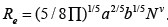
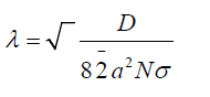
Polymers are linear macromolecular structures that are already known as building blocks of life. They are composed of repeating units of atoms or molecules. Each repeating unit of polymers are known as monomers. The connectivity throughout monomers is established via covalent bonds in which the valence electrons of atoms or molecules are shared together. The covalent bonds are among the strongest bonds in nature. The Brownian motion of monomers which arise from collisions by interstitial water molecules, causes monomers to fluctuate. The fluctuations of monomers makes the whole chainto undergo all possible configurations in the long time measurement. The average chain extension plus other time-averaged quantities are key properties of polymers that physicists seek. The end-to-end distance R_e and the radius of gyration R_g [1-3] are two candidates for average chain extension, however, R_g is more accurate.Simple calculations show that

. For pointlike monomers with no internal structure,

that is called freely-jointed-chain model (FJC). Where, N is the number of monomers i.e. degree of polymerization and a is the monomer size or the Kuhn length. In the FJC model, the monomers distribute by the Gaussian distribution. If we assume that monomers have internal structure, the monomers will interact via excluded volume interactions. All polymer Physics approaches including perturbation expansion theory (PET), renormalization group theory (RG), scaling theory (ST), mean field theory (MFT) and density functional theory (DFT) reveal that

. Where, b here denotes the second Virial coefficient and beers information about interactions between monomers. [1-3] The Flory exponent ν is equal to 3/5 or more precisely 0.588. [1-3] In essence, 1/ν is the fractal dimension of the linear polymer chains. [3] As the excluded volume interactions between monomers turns on, distribution of monomers gets parabolic. [1-3] One of the most interesting facts about polymers is that the average chain extension is a very sensitive function of molecular parameters, interactions between monomers and between monomers and solvent molecules. For instance, when the chain is suspended in a good solvent like water, b = 2.09 a³ so the chain swells, however, when it is suspended in a θ solvent b = 0 and the Gaussian model holds. [1-3] On the other hand, a polymer chain suspended in a poor solvent like Alcohol, feels b < 0 and chain collapses i.e.

. [1-3] One of the most applicable forms of polymers is a type of polymer solution in which the linear chains are grafted to a flat surface by one end. This system is known as polymer brushes and has been the subject of a huge number of researches in the last decades.

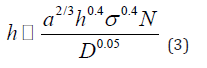
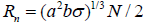
In this system, the steric repulsion among the monomers stretch the chains drastically in the perpendicular direction. The density functional theory (DFT) reveals that the average perpendicular chain extension in perpendicular direction or brush height is

and the mean lateral chain extension is the same as single isolated chain. [2,4] Polymer brush coated surfaces can have selfhealing properties and many others such as Glycol on the outside of the cell membrane and they play a key role in cells movement and interactions [2]. Nevertheless, here, I am interested in lubrication properties of two opposing brush covered surfaces that are located in the distance where the top and bottom chains intermediately interpenetrate. This system is known as polymer brush bilayer (PBB). [2,5-6] Schematic view of the PBB system at equilibrium and under stationary shear conditions are shown in Figure 1. The lubrication properties of the PBBs play a key role in the joints of humans and other mammals. The presence of aggregans in the synovial fluid of the mammalian joints are a good example. Recently, [4] there has been a tough competition on establishing a correct theory for the equation of state of the PBBs in equilibrium and under stationary shear [5,7-14], Many experiments has been also done to test lubrication properties of the PBBs [15-17].

In this article, I approach the PBBs theoretically and numerically. The theoretical part is done by a combination of the DFT framework and scaling theory. The numerical part is done by MD simulations. In the coming two sections, I briefly describe the theoretical part and in one section I describe the numerical simulation part. Finally, in the last section, I present the results and I discuss the results and conclude this research.

Low Shear Rate Scenario

One of the useful methods to study mechanics of a many body system is the DFT. In the DFT, the Euler-Lagrange equation of the system is calculated from a grand potential functional which is primarily based on a guess. There are also other methods such as Newton’s equation of motion and Hamilton-Jacobi method. In 1988, Hirz in his Master’s thesis applied the DFT method to polymer brush problem and obtained density profiles as well as brush height. [6] Following the same procedure that Hirz did, the PBBs grand potential functional could be given as follows,

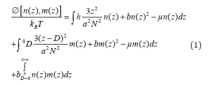
Where n(z) and m(z) are the density profiles of the bottom and up brushes respectively, [8] h the brush height, µ the chemical potential, σ the grafting density and D the distance between flat surfaces. Three Euler-Lagrange equations could be obtained plus one constraint which all are given as follows,

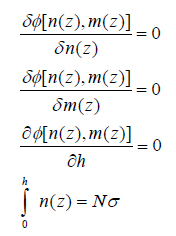
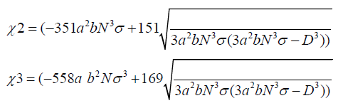
The first three equations say that equilibrium density profiles and height is calculated by setting functional derivatives of grand potential with respect to those quantities to zero. The last equation says that the total number of particles are fixed. To obtain equilibrium n(z), m(z), h and µ that are primarily unknown quantities, the four equations above need to be solved simultaneously because they are coupled to each other. The solutions of the above set of coupled equations are given as follows,

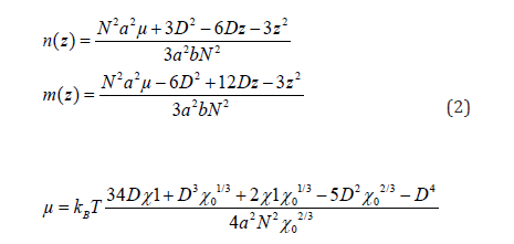
where χ₀ and χ₁ are volumes defined as follows,

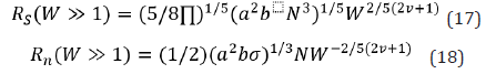
By plotting h as a function of each parameter, it turns out that h follows the following similarity relation,

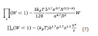
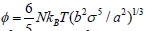
To calculate the equation of state of the PBBs, all calculated quantities are put back into Equation (1), and the pressure via the Gibbs-Dohem relation Φ = −PV is calculated. Thus, the equation of state of the PBBs is calculated as follows,

where the following volumes are defined,

By plotting the pressure equation, it could be simply inferred that the pressure follows the following similarity relation,

It turns out that, the equation [17] of state scales as (N/D)⁴ which is very important outcome and violates all previous calculations. [18] It reveals that pressure is strongly sensitive to N and D unlike single brush. The quadratic dependence of PBBs pressure on the degree of polymerization as well as distance between surfaces originates from complex interactions between monomers. The phenomenological arguments approaches a physical system by means of simple as- sumptions and obtains the general behavior of that system. The scaling theory is based on the phenomenological arguments and is capable of solving complex physical problems in a simple way. The problem of the PBB under shear seems to be very complicated at first sight. However, by using the following argument, it gets easier to solve. Upon shearing the PBB, above a critical shear rate, the chains start stretching in the shear direction. This is similar to the equilibrium condition but with chains stretched laterally. We can use this concept to build our scaling theory. I introduce a scaling function in the form of

the shear rate and v the relative velocity of surfaces. The goalis to calculate the exponent α. From DFT calculations, we know the physical quantities at low shear rates. The normal stress is the same as Equation. (4) and the shear stress is obtained by multiplying the viscosity by the shear rate. To calculate the viscosity, we need to look deep inside the system in the molecular scale. Each particle in the system, travels freely an amount of time τ between two subsequent collisions with another particle. The corresponding distance is called mean-free-path λ. From statistical Physics, it is known that for each system,

with n density of the system. [4] The average density of the PBBs is n = 2Nσ / D so the mean-free-path becomes,

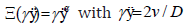
Again from statistical Physics, it is known that for each system

with v_rms the root-mean-squared velocity of particles. [4] For polymer chains, it is a bit tricky to calculate the root-mean-squared velocity. Since the monomers undergo Brownian motion,they perform diffusive movement rather than ballistic movement. For this reason, for polymer chains

with D_G the diffusion constant of the center of mass monomer. This literally means that every monomer diffuses the same as the center of mass monomer D_G. Later, I replace the appropriate D_G to calculate the λ and I obtain the corresponding τ. When the correct form of the τ is known for each type of system, the viscosity is obtained as τ γ˙. In the absence of hydrodynamic interactions (HIs), the polymer dynamics is governed by Rouse dynamics. [19] In this regime, when the shear rate exceeds a critical value, the shear forces dominate the fluctuation forces as well as the steric forces, and consequently, the chains start to stretch in the shear direction. In the Rouse’s dynamic, the critical shear rate is equal to inverse of

. Note that, this is the longest Rouse’s relaxation time.

For simplicity, it is useful to work with a dimensionless quantity W ÿ=τ Rγ instead of shearrate. This dimensionless quantity is called Weissenberg number. Now, in an step-by-step fashion, I calculate the physical quantities both in linear and non-linear regimes. The chain extensions at linear regime are given as follows,

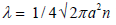
The diffusion constant of center of mass monomer in the Rouse’s dynamics with excluded volume interactions is given as

. 20 Therefore, the mean-free-time in this condition is given as follows,

The viscosity in the linear regime is

. Hence, the shear and normal stresses at the linear regime is obtained as follows,

Now, I utilize the scaling argument to calculate the physical quantities at non-linear regime i.e. when the shear forces dominate the fluctuation forces. When the shear rate exceeds the critical shear rate

, the shear extension must scale as N, similar to what the normal extension was in the equilibrium. This way, we determine the scaling function as

for the shear extension and

for the normal extension. Doing so together with some simplifications, we get the following similarity relations,

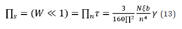
In the case of stress tensor, the scaling argument implies that the shear stress at non- linear regime, scales as N⁴. This way, I determine the scaling function for stresses as

. After doing simplifications, the following similarity relations obtained,

And finally, the kinetic friction coefficient at non-linear response regime is calculated via dividing shear stress by normal stress,

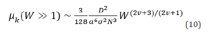
This is a very important result that we will see in the next sections that is in agreement with MD simulations results.

High Shear Rate Scenario

At high shear rate, the chains continue stretching in the shear direction up to a moment when the top and bottom brushes do not interpenetrate anymore. This is the moment when the normal extension equals half the wall distance. It means that when

which leads to the following shear rate,

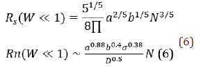
 At γ˙s the equation of state by which we had build our scaling theory is changed. This is completely different scenario with respect to previous one. So we need to do everything from the scratch. The equation of state in this condition is the equation of state of a single brush which is given as follows,

The equation above is calculated by using the grand potential of a single brush

, the Gibbs-Duhem relation

and the normal extension of a single brush

. On the other hand, the mean free path in this conditions is calculated as follows,

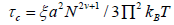
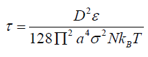
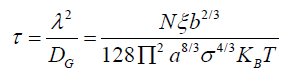
The mean free time is then calculated as follows,

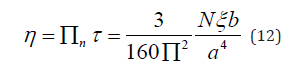
So we can now calculate the viscosity in this scenario as follows,

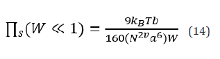
Thus the shear force in linear regime is given as follows,

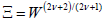
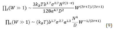
Now, we can use the scaling theory to check shear stress at high shear rates in this scenario. As before, we build an scaling function

and try to calculate α by considering the power of N. The phenomenological argument here is that when the chains are stretched in the shear direction, the shear stress must be proportional to N . This leads us to the equation 1+ (2ν +1)α=1 which gives us α = 0. This tells us that in the no-interpenetration scenario the shear stress is given as following,

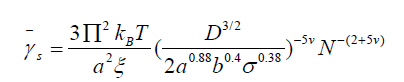
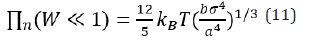
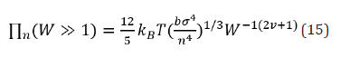
The normal stress is obtained by using the fact that it must become proportional to N³ at high shear rate. This leads us to the equation  which clearly gives us α = −1/ (2ν + 1). Therefore, the normal stress in this scenario is given as follows,

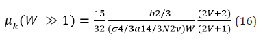
Hence, the kinetic friction coefficient in this scenario becomes the following relation,

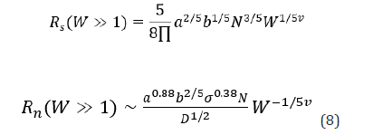
Repeating the same procedure for the chain extensions, we get the following equations

for the shear and normal chain extensions,

Molecular Dynamic Simulation

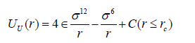
The molecular dynamic simulation is based upon calculation of trajectories of each particle in a discrete manner. The trajectories of each particle is calculated from the Newton’s equation of motion. In the present research, I use the Leap-Frog algorithm to discrete the equations of motion of monomers. This scheme calculates trajectories of monomers with a accuracy of the order of magnitude ∆ t⁴ which is very precise. It also allows for using large time step and faster calculations. In the simulations, the system is composed of two surfaces located at z = 0 and z = D. The surfaces are build by arranging atoms in a 2D simple cubic lattice. The area of the surfaces is L_x = 20σ times L_y = 20σ . The linear polymer chains of degree N are grafted to randomly chosen wall atoms. The periodic boundary conditions (PBC) is employed to mimic the bulk properties in the system. The shear motion is produced by moving the bottom wall atoms in the +y direction and the top wall atoms in the −y direction with speed v/2. The Lennard-Jones potential which make the hard-core excluded volume interactions between particles is given as follows,

And the finitely-extensible-nonlinear-elastic (FENE) potential connects the monomers in the chains is given as follows,

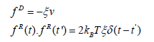
The Langevin thermostat is given as follows,

In the coarse-grained simulation all quantum mechanical degrees of freedom are inte- grated. It is called Kremer-Grest model. [20,21] The simulations have run for 10⁵ time steps and to capture the most accurate results. Table 1 shows the numerical values of simulation parameters in my simulation.

Results and Conclusion

The problem of the PBBs under stationary shear motion is studied by means of the DFT framework, the scaling theory and the MD simulations. In Figure 2(i), the shear force exerted on the top wall in terms of the shear rate is shown. Here, the similarity relation Equation. (9) for the shear force in non-linear regime of the low shear scenario, Equation. (14) for the shear force in non-linear regime of the high shear scenario and the MD simulations results are shown together. As it is seen, the shear force scales as γ˙^1.46 in low shear rate scenario where the brushes interpenetrate and it scales as γÿ^−0.46 .˙ in high shear rate scenario where the brushes do not interpenetrate. In Figure 2(i), we see a perfect agreement between the DFT and the MD simulations. Each plot shows the DFT and the MD simulations results at low and high shear rate scenarios. In Figure 2(ii), the normal force exerted on the top wall in terms of the shear rate is shown. Here, the similarity relation Equation. (9) for the normal stress of the low shear scenario, Equation (15) for the normal stress in high shear scenario and MD simulations results are shown together. It is shown that the normal stress at both low and high shear scenario scales as . Here again, we see a great agreement between DFT and MD simulations. In Figure 2(iii), the kinetic friction coefficient for both scenarios are shown. Here, the similarity relation Equation. (10), Equation. (16) and the MD results are shown. It turns out that the kinetic friction coefficient at low shear scenario scales as γÿ^1.92 and at high shear scenario scales as γÿ^1.46 . We find a great agreement between the DFT and the MD simulations. In Figure 2(iv), the shear viscosity in terms of the shear rate is shown. Note that the shear viscosity could be calculated by dividing the shear force in each scenario by the shear rate.

It turns out that the shear viscosity scales as γÿ^0.46 at low shear scenario and it is independent of the shear rate at high shear scenario. These universal power laws are well confirmed by the MD simulations as well. In Figure 2(v), we see the shear chain extension in terms of the shear rate. Here, the MD simulations results reveal an anomalous behavior of chains in the shear direction. It turns out that by increasing the shear rate, the shear chain extension increases, then decreases and again increases. Apparently, when we increase the shear rate, there is a critical shear in which the chains have minimum extension in the shear direction. This critical shear rate could be the topic of more researches in the future. And finally Figure 2(vi) shows the normal extension of the chains in terms of the shear rate. Here, we see Equation. (8), Equation. (17) and the MD simulations results together. It turns out that the normal extension at low shear scenario scales as γÿ^−0.34 while at high shear scenario, it scales as γÿ^−0.18 As it is seen, we again get a great agreement between the DFT and the MD simulations results. Without any complicated calculations or extensive numerical simulations, one immediately infers that when two opposing polymer brushes intermediately compressed such that their chains interpenetrate into each other, the friction between them is larger than simple fluids. The reason is clear the interpenetrating chains produce larger friction.

However, to find out the power laws we must use theoretical tools. So, my theoretical approach predicts that when two interpenetrating brushes are sheared, the shear stress scales as γÿ^1.46 , of course, as long as the brushes interpenetrate. This universal power law is very important because it correctly shows that if we use the equation of state of the polymer brush bilayer with interpenetrating chains, and apply the scaling theory to this equation of state, we get the correct power law. This is really amazing because molecular dynamic simulations confirm this power law as well. The second scenario takes place when the chains stretch drastically in the shear direction such that eventually the normal chain extension reaches D/2 and at this moment the interpenetration zone vanishes. At this moment, the equation of state is changed and we have to apply the scaling theory to the equation of state of a single brush or non-interpenetrating brushes which are equal in meaning. When we do the same procedure

 on this equation of state, we surprisingly get the power law γÿ for the shear stress. This is really really amazing because both theory and simulations strongly agree on this scenario. In conclusion, the interpenetration between top and bottom brushes play the key role in the behavior of the system. If we take into account the explicit solvent molecules, it is always and in any conditions the solvent molecules concentrate in the middle of brushes and push the brush monomers out of the middle zone. It means that with explicit solvent molecules we never ever have an interpenetration zone between brushes. Note that you cannot reach any interpenetration by compressing the brushes over each other because the solvents are always there. Therefore, with explicit solvents, the shear stress always scales linearly with the shear rate. It means that there is no sublinear regime in the PBB system. Hence, at the end of this article I would say that the works already published [5,13-15] are completely wrong.

Acknowledgment

It is my honor to acknowledge the Biomedical Journal of Scientific and Technical Research (BJSTR) for supporting my research. Also, I am honored to acknowledge the Cold Spring Harbor Laboratory (CSHL) and the Regeneron Pharmaceuticals Inc. [22-26] for giving credit to my research. I also, thank Weizmann institute for the XMGrace software, the Wolfram Research for the Mathematica software and the GNU Inc. for the GFortran without which my research was not come into reality.

References

1. Rubinstein M, Colby RH (2003) Polymer Physics. OUP Oxford.
2. Gennes, Pierre Gilles (1979) Scaling Concepts in Polymer Physics. Cornell University Press, p. 74-75.
3. Safran S (2003) Statistical Thermodynamics of Surfaces, Interfaces, and Membranes. Boca Raton CRC Press, pp. 288.
4. Klein Jacob, Kumacheva Eugenia, Mahalu Diana, Dvora P, Lewis JF (1988) Reduction of frictional forces between solid surfaces bearing polymer brushes. Nature 370(6491): 634-636.
5. Azzaroni O, Szleifer I (2017) Polymer and Biopolymer Brushes, for Materials Science and Biotechnology Volume Set.
6. Lilge I (2017) Polymer Brush Films with Varied Grafting and Cross-Linking Density via SI- ATRP. Analysis of the Mechanical Properties by AFM Springer Fachmedien Wiesbaden.
7. GB Arfken, HJ Weber, FE Harris (2013) Mathematical methods for Physicists, a comprehensive guide, Elsevier.
8. Schwabl F, Brewer WD (2006) Statistical Mechanics, Advanced Texts in Physics, Springer Berlin Heidelberg, pp. 313-316.
9. Kreer T (2016) Polymer-brush lubrication: a review of recent theoretical advances. Soft Matter 12: 3479-3501.
10. Hirz SJ (1988) Modeling of Interactions Between Adsorbed Block Copolymers, University of Minnesota, Minneapolis, MN.
11. MILNER ST (1991) Polymer Brushes. Science 251(4996): 905-914.
12. Halperin A, Tirrell M, Lodge TP (1992) Tethered chains in polymer microstruc-tures. Macromolecules: Synthesis, Order and Advanced Properties, Springer Berlin Heidelberg, Berlin, Heidelberg, p. 31-71.
13. Szleifer I, Carignano MA (2007) Wiley-Blackwell, Tethered Polymer Layers. Advances in Chemical Physics, pp. 165-260.
14. Milner ST, Witten TA, Cates ME (1988) A Parabolic Density Profile for Grafted Polymers. EPL (Europhysics Letters) 5(5): 413.
15. Zhulina EB, Borisov OV (1991) Structure and stabilizing properties of grafted polymer layers in a polymer medium. Journal of Colloid and Interface Science 144(2): 507-520.
16. Galuschko A, Spirin L, Kreer T, Johner A, Pastorino C, et al. (2010) Frictional Forces between Strongly Compressed, Nonentangled Polymer Brushes; Molecular Dynamics Simulations and Scaling Theory. Langmuir 26(9): 6418-6429.
17. Kreer Torsten, Binder Kurt, Müser Martin H (2003) Friction between Polymer Brushes in Good Solvent Conditions, Steady-State Sliding versus Transient Behavior. Langmuir 19(18): 7551-7559.
18. Mittal V (2012) Polymer Brushes, Substrates, Technologies, and Properties, CRC Press.
19. Kreer T, Müser MH, Binder K, Klein J (2001) Frictional Drag Mechanisms between Polymer-Bearing Surfaces. Langmuir 17(25): 7804-7813.
20. Klein Jacob, Perahia Dvora, Warburg Sharon (1991) Forces between polymer- bearing surfaces undergoing shear. Nature 352(6331): 143-145.
21. Taunton HJ, Toprakcioglu C, Fetters, Lewis J, Klein J (1988) Forces between surfaces bearing terminally anchored polymer chains in good solvents. Nature 332: 712-714.
22. Advincula RC, Brittain WJ, Caster KC, Rühe J (2004) Polymer Brushes, Wiley-VCH, Weinheim.
23. Doi M, Edwards SF (1986) Theory of polymer dynamics. Oxford science publication.
24. Smit B, Frenkel D (1996) Understanding Molecular Simulation: From Algorithms to Applications, Academic Press.
25. Kremer K, Gres GS (1990) Dynamics of entangled linear polymer melts: A molecular- dynamics simulation. The Journal of Chemical Physics 92: 5057-5086.
26. Edwards M (2018) Polymer brush bilayers at thermal equilibrium: A theoretical study.