The Use of Artificial Intelligence in the Classification of Medical Images of Brain Tumors Volume 53- Issue 4

Marcos A M Almeida* and Matheus H C de Araujo

• Department of Electronics and Systems, Technology Center, Federal University of Pernambuco, Brazil

Received: October 05, 2023; Published: November 14, 2023

*Corresponding author: Marcos A M Almeida, Department of Electronics and Systems, Technology Center, Federal University of Pernambuco, Recife-PE 50670-901, Brazil

DOI: 10.26717/BJSTR.2023.53.008450

Abstract PDF

ABSTRACT

Early detection in diagnosing brain diseases is crucial for proper disease treatment measures. The use of Artificial Intelligence/Machine Learning has contributed to the classification of diseases through medical images. Algorithms, models, and increasingly powerful techniques have emerged to assist physicians in this decision-making process. This research proposes to classify medical images using pretrained neural networks. The VGG16 model outperformed the other studied models, including VGG19, InceptionResNetV2, and InceptionV3. Models were evaluated by brain disease class, which included notumor, pituitary, glioma, and meningioma. The metrics used to evaluate the models included accuracy, precision, sensitivity, and specificity, all registering values above 95%. Furthermore, the Diagnostic Odds Ratio was above 473.00, indicating excellent responses based on the medical images. Overall, the results suggest that Artificial Intelligence techniques have made significant contributions to the early diagnosis of brain tumors.

Keywords: Artificial Intelligence; Image Classification; Neural Networks; Computer Vision; Transfer-Learning; Medical Image Analysis

Introduction

Brain tumor cases increased significantly globally between 2004 and 2020 from nearly 10% to 15% [1]. The early detection and diagnosis of brain tumors are crucial for taking appropriate preventive measures, as is the case with most cancers [2]. Recent advancements in using artificial intelligence resources for diagnosis using medical images have greatly facilitated image classification. Javaria Amin, et al. [3] describe and present results of several scientific methods to detect and classify brain tumors using traditional techniques such as thresholding and growth variations in the region of interest. Additionally, the use of data extraction techniques from 2D/3D medical images of human tissues suspected of tumors and the use of Artificial Intelligence/Machine Learning techniques are efficient for the detection of these tumors through the analysis of these images. In the era of molecular therapies, diagnostic neuroimaging should guide the diagnosis and treatment planning of brain tumors through a non-invasive characterization of the lesion, sometimes also called “virtual biopsy”, based on radiomic and radiogenomic approaches [4,5]. The tumor is an exceptional expansion generated by human cells that reproduce abnormally. Identifying brain tumors is crucial, and changes in tissue color and texture can help with their diagnosis from images. Texture, which includes attributes like brightness, color, and size, can be partitioned into sub-images for analysis. This analysis can provide valuable insights into classifying the tumors and extracting vital information from the images [6]. Additionally, intrinsic image alterations like brightness and color can aid texture analysis and further differentiate the images. A sample of the images is displayed in Figure 1.

Materials and Methods

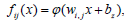
The studied models are known in the academic literature and are part of the set of discriminative models. Deep learning algorithms applied in computer vision, and when used in medical images, take this technology to a sophisticated level of feature extraction to the point of classifying diseases through these images. The Artificial Intelligence/Machine Learning tools used in this study are Convolutional Neural Networks [7], where a L-layer neural network is a mathematical function S, called feature map, which is a composition of multivariate functions: f_1,1, ..., f_i,j, ..., f_n,L , and K_i,j, is defined as:

where,

• n is the dimension of the input x.

• p is the dimension of the output of the last layer.

• L is the number of layers.

• K is the filter or kernel function.

• each function is itself a composed multivariate function

where ϕ(.) is the activation function, w represents the weights, and b is the bias.

The models studied follow the basic configuration of the graphical representation which is shown in Figure 2.

The feature map in discrete form S_i,j is expressed by Equation 2:

where, M is the kernel dimension.

Equation 3 shows the 2D layer of a Convolutional Neural Network.

where, z is the kernel filter order.

The models taken into consideration in this study have structures based on the configuration shown in Figure 2, whose composition and order of layers for each model are shown in subsection Proposed Strategy and have layers with the following characteristics:

• 2D Convolutional filter;

• Batch Normalization;

• ReLu;

• Full Connected;

• Average Pooling;

• Max Pooling;

• Dropout;

Proposed Strategy

Our research proposes a combination of methods and techniques that can achieve great results in image classification. Through these techniques, we can identify and distinguish various human tissue structures to detect different diseases. Data were collected from an online source available on the kaggle.com platform [8], where the data set was processed, which was divided into two groups: 66.66% for training and 33.37% for validation. Four different types of brain imaging were classified: no-tumor, pituitary tumors, glioma tumors, and meningioma tumors. This research utilized a dataset of 600 brain tumor images for multiclass classification. For each of the simulated models, the input images for the convolutional layer are fixed-size 3x128x128 RGB images, resized from original brain images in 600-pixels jpeg format, [8]. The randomly selected images were passed through a stack of convolutional layers with the most diverse functions for feature extraction. The architectures were modeled using the Python language with the Keras and Tensor-Flow libraries in Python environment. The experimental design took into account the following parameters and simulation settings to facilitate the extraction of features from each image: the data augmentation method was applied to increase the brightness and contrast of the images. The optimized used was the ADAM algorithm, with a learning rate of 0.0001, and the loss function used was the "sparse categorical cross-entropy", this metric uses two local variables, total and count that are used to calculate the frequency with which ypred corresponds to ytrue, used for model training.

One of the methods applied was the transfer of learning [9], which transfers the optimized weights of the original neural networks to the new model structure. This approach, as explained by Peirelinck, et al. [10], is a powerful tool for achieving accurate image classification. The results plotted in Figure 3 show the difference with transfer and without transfer learning and the impact on the models’ performance. This research proposes the extraction of features from medical images of brain diseases, from a pre-processing of the images, and in the sequence of the training phase. The trained model was submitted to the testing phase when the results of the metrics by class or type of disease were obtained. The layer diagram of models VGG16 and VGG19, as shown on Figure 4. Models VGG16 and VGG16 have similar structures, where each block is composed of 2D Convolution and Max Pooling layers, with 16 and 19 layers, respectively. Figure 5 presents the InceptionResV2 and InceptionV3 models. InceptionV3 is an image recognition model that achieves over 78.1% accuracy on the ImageNet dataset. This model is the culmination of many ideas developed by several researchers over the years. It is based on the original paper “Rethinking the Inception Architecture for Computer Vision" [11]. The steps of the Inception process are convolution, pooling, dropout, fully connected, and softmax [12,13].

Metrics for Evaluating Models

The studied models were evaluated using the following set of metrics:

• TP = True Positive;

• FP = False Positive;

• TN = True Negative;

• FN = False Negative;

• P = Total Positive;

• N = Total Negative,

where,

where P and N indicate the number of positive and negative samples, respectively.

1) Accuracy and error rate Accuracy (Acc) is one of the most commonly used measures for classification performance, and it is defined as a ratio between the correctly classified samples to the total number of samples as follows [14], according to Eq. 6:

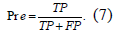
2) Precision (Pre) is a metric that quantifies the number of correct positive predictions made. Precision, therefore, calculates the accuracy for the minority class. It is calculated as the ratio of correctly predicted positive examples divided by the total number of positive examples that were predicted, according to Eq. 7:

3) Sensitivity, True Positive Rate (TPR), hit rate, or recall, of a classifier represents the positive correctly classified samples to the total number of positive samples. The sensitivity measures the capability of the diagnostic test to recognize a diseased person correctly [14], i.e., S+ = Pr(test positive/non−diseased) = , where is the error probability of falsely classifying a diseased person as healthy, or even as defined in Eq. 8:

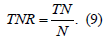
4) Specificity, True Negative Rate (TNR), represents the negative correctly classified samples to the total number of negative samples. The specificity measures the capability of diagnosing a healthy person correctly [14], i.e., S− = Pr(test negative|non-diseased) = (1-), where is the error probability of falsely classifying a healthy person as diseased, or even as defined in Eq. 9:

In some situations, sensitivity has precedence over specificity, for instance, to assess the clinical utility of prognostic biomarkers in cancer [15].

5) F1-Score or F1 measure is a performance metric that represents the harmonic mean of precision and recall as in Eq. 10 [16,17]. The value of the F1-measure is ranged from zero to one, and high values of the F1-measure indicate high classification performance. F1 Score is the Harmonic Mean between precision and recall and the Precision is the proportion of true positives among instances classified as positive, e.g. the proportion of melanoma correctly identified as melanoma. Recall is the proportion of true positives among all positive instances in the data, e.g. the number of sick among all diagnosed as sick.

6) Matthews Correlation Coefficient (MCC) represents the correlation between the observed and predicted classifications [16,18], and it is calculated directly from the confusion matrix as in disagreement between prediction and true values and zero means that no better than Eq. 11:

A coefficient of +1 indicates a perfect prediction, −1 represents total disagreement between prediction and true values and zero means that no better than random prediction.

7) Cohen’s Kappa measures the agreement between two raters who classify N items into C mutually exclusive categories [19], according to Eq. 12:

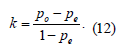
where p_o is the observed relative agreement between raters and p_e is the hypothetical chance of agreement by chance, using the observed data to calculate the odds of each observer randomly viewing each category. Cohen’s kappa is a robust statistic useful for either interrater or intrarater reliability testing.

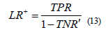
8) Positive Likelihood Ratio (LR)+ combines both sensitivity and specificity, and it is used in diagnostic tests [14]. Positive likelihood - LR+ measures how much the odds of the disease increase when a diagnostic test is positive and it is calculated as in Eq. 13:

9) Negative Likelihood Ratio (LR)− combines both sensitivity and specificity, and it is used in diagnostic tests [14]. Negative likelihood - LR− measures how much the odds of the disease decrease when a diagnostic test is negative and it is calculated as in Eq. 14:

10) Diagnostic Odds Ratio (DOR) has been suggested and utilized frequently in the literature. The diagnostic odds ratio as a single indicator of diagnostic performance, as proposed and recommended for example by Glas, et al. [15], and is defined as Eq. 15. The value of a DOR ranges from 0 to infinity, with higher values indicating better discriminatory test performance. A value of 1 means that a test does not discriminate between patients with the disorder and those without it.

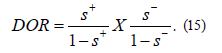
In fact, the original paper by Glas, et al. [20], suggested the DOR as a single indicator of test performance to facilitate the formal meta-analysis of studies on diagnostic test performance.

11) Confusion Matrix (CM) is a fundamental tool in machine learning and statistics that is used to evaluate the performance of a classification algorithm. It provides a visual representation of the performance of a classification model by summarizing the predictions it has made on a dataset and comparing them to the actual known labels. The confusion matrix is particularly useful when dealing with binary classification problems (two classes) but can also be extended to multiclass classification problems. The confusion matrix provides a comprehensive overview of the model’s performance, allowing for deeper insights into its strengths and weaknesses.

12) Receiver Operating Characteristics (ROC) curve is a two-dimensional graph in which the TPR represents the y-axis and FPR is the x-axis. The ROC curve has been used to evaluate many systems such as diagnostic systems, medical decision-making systems, and machine learning systems [16]. It is used to make a balance between the benefits, i.e., true positives, and costs, i.e., false positives, as shown in Figure 6.

Results and Discussions

It can be observed that for each model, certain types of disease are more easily identified than others, this is justified by the fact that some of the studied models manage to extract more characteristics from others. In the simulation of the studied models, pre-trained and trainable parameters were used, according to Table 1. These CNNs have been trained on the ILSVRC-2012-CLS image classification dataset [21].

VGG16 Model Evaluation

Among the analyzed models, the VGG16 model is one of the models that have fewer parameters to be trained, however, the model presents good results shown in Table 2. This model shows greater ease in identifying the image of a pituitary, with an accuracy of 95.50%, and a diagnostic odds ratio (DOR) of 462.00, as well as, notumor with an accuracy of 94.50% and a DOR of 268.66. However, it presents some difficulty in identifying the disease meningioma with an accuracy of 88.00%, a Mattheus Correlation Coefficient of 59.35%, and a DOR of 25.33. Mahmud, et al. [1] worked with a data set that was divided into three groups: 80% for training, 10% for testing, and 10% for validation. It validated four different types of brain imaging: glioma tumors, meningioma tumors, no-tumor, and pituitary tumors, in a total of 3,264 images. Found for the VGG16 model an accuracy of 71.60%. Figure 7 shows for each class the number of test images that were correctly and erroneously predicted through the confusion matrix. It is observed that the VGG16 model classifies pituitary disease more easily. The ROC curve confirms in the binary classification that the pituitary instance is the most prevalent with an AUC of 96%, and the lowest is the meningioma with an AUC of 80%, as shown in Figure 8.

VGG19 Model Evaluation

For the pre-trained model VGG19, the best classification was with no tumor images, with an accuracy of 93.50%, precision of 95.65%, and a DOR of 172.86. Table 3 shows these results. The results presented in Table 3 for the VGG19 model are generally lower than the results for the VGG16 model shown in Table 2. Using the aggregation technique of robust CNN, Anaya Isaza, et al. [2] obtained image classification results with the VGG19 model, an accuracy of 76.76%, with a precision of 89.29% (Figure 9).

InceptionResNetV2 Model Evaluation

The InceptionResNetV2 model did not show a good response in the diagnostic identification of the images considered in this study, due to the results of the metrics presented in Table 4. The InceptionResNetV2 model presents the best classification for non-tumor images, with an accuracy of 93.50%. Obtaining accuracy and precision values of 96.78% and 97.67%, respectively, with the InceptionResNetV2 model, Gómez Guzmán, et al. [22] reached a great level in the validation metrics of this model. The InceptionResNetV2 model presents a good response in the identification of meningioma diagnostic imaging, better than the VGG19 and InceptionV3 models, with an AUC of 76% as shown in Figures 10 & 11.

InceptionV3 Model Evaluation

The InceptionV3 model responds well to the identification of non-tumor images, with an accuracy of 95.00%. Gómez Guzmán, et al. [22] included in their research the pre-trained model InceptionV3 with a total of 5,712 images for training and 1,311 for testing. The experimental results showed an accuracy of 97.12% and a precision of 97.97%, obtaining excellent results. The Confusion Matrix in Figure 12 shows that the InceptionV3 model has a better performance for non-tumor classification and a poor performance for identifying meningioma images. In this study, considering the test database, the AUC of the InceptionV3 model reached levels between 93% and 69%, according Figure 13. The pre-trained models InceptionResNetV2 and InceptionV3, in general, presented average performance, below the models VGG16 and VGG19. After carrying out a thorough analysis, it was found that the VGG16 model had the strongest overall performance when compared to the studied models (Table 5).

Conclusion

In this research, the use of models with pre-trained parameters is a highly effective solution, not only significantly improving the processing response time in the classification of medical images, but also producing very satisfactory results. These findings suggest that the use of pre-trained models can be a valuable tool in the field of medical image analysis for the early identification of diseases. Out of the four models evaluated for identifying images with diseases like pituitary type, glioma, and meningioma, the VGG16 model stood out with the best performance. Based on our evaluation of four different models, we found that the VGG16 model performed the best in identifying images with pituitary-like disease, glioma, and meningioma. This model provided very good results in accuracy, precision, sensitivity/retrieval, specificity, and Matthews correlation coefficient. However, when it comes to detecting no-tumor images, the InceptionV3 model was the best model,

evaluated with a Matthews correlation coefficient of 88.54%, sensitivity/recall of 98.52%, and diagnostic Odds Ratio of 473.81. The VGG16 model emerges as the second-best model to detect no-tumor images, but the InceptionV3 model was the absolute leader in this category. Based on the set of images presented, the research showed that meningioma is the most difficult disease to classify among the four studied models. Classification accuracy ranged from 77.00% to 88.00%

Author Contributions

The first author contributed to the writing of this article and part of the simulation. Matheus H. C. de Araújo contributed to part of the simulation. All authors have read and agreed to the published version of the manuscript.

Funding

Not Applicable.

Institutional Review

Not Applicable.

Disclosure

The authors declare no conflict of interest.

Acknowledgment

We would like to thank Kaggle (kaggle.com) for making databases of brain disease images publicly available.

References

1. Mahmud MI, Mamun M, Abdelgawad A (2023) A Deep Analysis of Brain Tumor Detection from MR Images Using Deep Learning Networks. Algorithms 16(4): 01-19.
2. Anaya Isaza A, Mera Jime´nez L, Verdugo Alejo L, Sarasti L (2023) Optimizing MRI-based brain tumor classification and detection using AI: A comparative analysis of neural networks, transfer learning, data augmentation, and the cross-transformer network. European Journal of Radiology Open 10: 01-12.
3. Amin J, Sharif M, Haldorai A, Yasmin M, Nayak RS (2022) Brain Tumor Detection and Classification using machine learning: a comprehensive survey. Springer Comp & Intell Syst 8: 3161-3183.
4. Cè M, Irmici G, Foschini C, Danesini GM, Falsitta LV (2023) Artificial Intelligence in Brain Tumor Imaging: A Step toward Personalized Medicine. Current Oncology-MDPI 30(3): 2673-2701.
5. Vagvala S, Guenette JP, Jaimes C, Huang RY (2022) Imaging Diagnosis and Treatment Selection for Brain Tumors in the Era of Molecular Therapeutics. Cancer Imaging 22(19): 01-14.
6. Almeida MAM, Santos IAX (2020) Classification Models for Skin Tumor Detection Using Texture Analysis in Medical Images. Journal of Imaging 6(51): 01-15.
7. Cabello JG (2022) Mathematical Neural Network Axioms. Axioms 11(2): 01-18.
8. (2023) www.kagle.com.
9. Zhuang F, Qi Z, Duan K, Xi D, ZhuY, et al. (2020) A comprehensive survey on transfer learning. Proc IEEE 109(1): 43-76.
10. Peirelinck T, Kazmi H, Mbuwir BV, Hermans C, Spiessens F Suykens J, et al. (2022) Transfer learning in demand response: A review of algorithms for data-efficient modeling and control. Energy 7(100126): 43-76.
11. Szegedy C, Vanhoucke V, Ioffe S, Shlens J (2015) Rethinking the Inception Architecture for Computer Vision. arXiv 1512.00567 cs CV, p. 01-10.
12. Andrew A, Santoso H (2022) Compare VGG19, ResNet-50, Inception-V3 for review food rating. Tek Inform 7(2): 845-494.
13. Al Husaini MAS, Habaebi MH, Gunawan TS, Islam MR, Elsheikh EA, et al. (2022) Thermal-based early breast cancer detection using inception V3, inception V4 and modified inception MV4. Neural Computing Applied 34(1): 333-348.
14. Chatzimichail T, Hatjimihail A T (2021) A Software Tool for Calculating the Uncertainty of Diagnostic Accuracy Measures. Diagnostics 11(406): 1-36.
15. Bohning D, Patilea V, Heinz Holling (2011) A limitation of the diagnostic-odds ratio in determining an optimal cut-off value for a continuous diagnostic test. Statistical Methods in Medical Research 20(5): 541-550.
16. Tharwat A (2021) Classification assessment methods. Applied Computing and Informatics 17(1): 168-192.
17. Sokolova M Japkowicz N, Szpakowicz S (2006) Beyond accuracy, f-score, and roc: a family of discriminant measures for performance evaluation. 19Th Australian Joint Conference on Artificial Intelligence Hobart Australia, pp. 1015-1021.
18. Chicco D, Totsch N, Jurman G (2021) The Matthews correlation coefficient (MCC) is more reliable than balanced accuracy, bookmaker informedness, and markedness in two-class confusion matrix evaluation. BioData Mining, p. 1-22.
19. McHugh ML (2012) Interrater reliability: the kappa statistic. Biochemia Medica (Zagreb) 22(3): 276-282.
20. Glas A S, Lijmer JG, Prins MH, Bonsel GJ, Bossuyt PMM (2003) The diagnostic odds ratio: a single indicator of test performance. Journal of Clinical Epidemiology 56(11): 1129-1135.
21. (2023) https://www.image-net.org/challenges/LSVRC/index.php.
22. Gómez Guzmán MA, TotschJiménez Beristaín L, García Guerrero E E, López Bonilla O R, Tamayo Perez U, et al. (2023) Classifying Brain Tumors on Magnetic Resonance Imaging by Using Convolutional Neural Networks. Electronics 12(955): 1-22.