On Stability of One Mathematical Model of the Epidemic Spread Under Stochastic Perturbations Volume 53- Issue 3

Leonid Shaikhet*

• Department of Mathematics, Ariel University, Ariel 40700, Israel

Received: September 09, 2023; Published: October 18, 2023

*Corresponding author: Leonid Shaikhet, Department of Mathematics, Ariel University, Ariel 40700, Israel

DOI: 10.26717/BJSTR.2023.53.008392

Abstract PDF

ABSTRACT

This paper continues the study of the asymptotic properties of the known SAIRP epidemic model under stochastic perturbations. The SAIRP epidemic model is described by a system of five nonlinear differential equations. It is assumed that the system is influenced by stochastic perturbations that are of the type of white noise and are proportional to the deviation of the current system state from one of the system equilibriums. It is shown that sufficient conditions of stability in probability for two different equilibria of the considered system are formulated via a simple linear matrix inequality (LMI), that can be easily studied via MATLAB. Two demonstrative examples illustrate the obtained results via numerical simulation of solutions of the considered system of five nonlinear Ito’s stochastic differential equations. The research method used here can be applied to a lot of other more complicated models in different applications.

Keywords: Equilibria; Stability in Probability; Asymptotic Mean Square Stability; Lyapunov Function; Linear Matrix Inequality (LMI); Numerical Simulation

Introduction

During the last years investigations of epidemic models are very popular in research (see, for instance, [1-3] and the references therein). The so-called SAIRP epidemic model is defined by the following system of ordinary differential equations [1]:

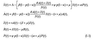
Here it is supposed that the population is subdivided into five distinct classes: susceptible individuals (S(t)); asymptomatic infected individuals (A(t)); active infected individuals (I(t)); removed (R(t)); protected individuals (P (t)). The total population, N (t) = S(t) + A(t) + I(t) + R(t) + P (t), with t ≥0 has a variable size, where the recruitment rate Λ and the natural death rate µ are assumed to be constant. The susceptible individuals S(t) become infected by contact with active infected I(t) and asymptomatic infected individuals A(t), at a rate of infection

where θ represents a modification parameter for the infectiousness of the asymptomatic infected individuals A. It is supposed also that all parameters of the system (1.1) are positive and, besides, p < 1, u < 1.

In [1] some properties of stability of the system (1.1) equilibria are studied. Below, following the method from [4], stability in probability of two equilibria of the system (1.1) is investigated by the assumption that the system (1.1) is exposed to stochastic perturbations that are of the type of the white noise and are directly proportional to the deviation of a system state from an appropriate equilibrium.

Equilibria

Assuming that all variables in the system (1.1) are constants, we obtain that the equilibria of the system (1.1) are defined by the system of algebraic equations

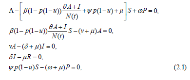
with the solutions: disease-free equilibrium

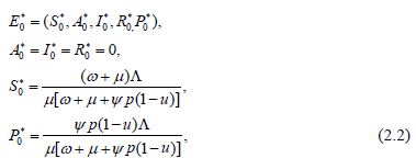
and endemic equilibrium

where the basic reproduction number R₀ > 1,

Note also that, summing all equations of the system (2.1), we obtain

for both equilibria (2.2) and (2.3).

Stochastic Perturbations

Let {Ω, 𝔉, P} be a complete probability space, {𝔉_t, t ≥ 0} be a nondecreasing family of sub-σ-algebras of 𝔉, i.e., 𝔉_t1 ⊂ 𝔉_t2 ⊂ 𝔉 for t₁ < t₂, E be the mathematical expectation with respect to the measure P.

Let us suppose that the system (1.1) is exposed to stochastic perturbations that are of the type of the white noise and are directly proportional to the deviation of the system state (S(t), A(t), I(t), R(t), P (t)) from one of the equilibria (S*, A*, I*, R*, P*). As a result, we obtain the system of Ito’s stochastic differential equations [5]

where σ₁, ..., σ₅ are constants and w₁(t), ..., w₅(t) are the mutually independent 𝔉_t -adapted standard Wiener processes.

Note that the equilibrium (S*, A*, I*, R*, P*) of the deterministic system (1.1) is also the solution of the system of Ito’s stochastic differential equations (3.1). Stochastic perturbations of this type were first proposed in [6] for SIR epidemic model and later also for a lot of other different applied models (see [7] and the references therein).

Centralization and Linearization

Consider the nonlinear differential equation

where x(t) ∈ Rⁿ and the equation F(x) = 0 has a solution x^∗ that is an equilibrium of the differential equation (4.1). Using the new variable y(t) = x(t) − x^∗, represent the equation (4.1) in the form

It is clear that stability of the zero solution of the equation (4.2) is equivalent to stability of the equilibrium x* of the equation (4.1).

Let

be the Jacobian matrix of the function

and

where

is the Euclidean norm in Rⁿ. Using Taylor's expansion in the form

and the equality F(x*) = 0, we obtain the linear approximation

of the nonlinear differential equation (4.2). So, a condition for the asymptotic stability of the zero solution of the linear equation (4.3) is also a condition for the local stability of the equilibrium x* of the initial nonlinear equation (4.1).

To construct the linear approximation of the system (3.1) let us put (′ is the sign of transpose)

Representing the system (1.1) in the form (4.1) and calculating the Jacobian matrix, we get the linear part of the system (3.1) in the form.

where B_i is the matrix with all zero elements besides of b_ii = σ_i, i = 1,…5, and

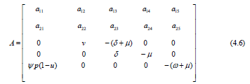
with

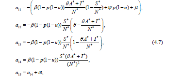
and

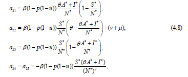
In particular, for the equilibrium E^∗₀ the elements (4.7) and (4.8) of the matrix (4.6) are

and

Remark 1 Let V = V (z) be a twice differentiable function of z∈R⁵. The generator of the equation (4.5) has the form [5]

Stability

Definition 1

Put y(t) = (S(t), A(t), I(t), R(t), P(t))-(S*, A*, I*, R*, P*). The solution (S*, A*, I*, R*, P*) of the system (3.1) is called stable in probability if for any  there exists   such that y(t) satisfies the condition

for any y(0), such that P{ y(0) <δ } =1

Definition 2

The zero solution of the equation (4.5) is called:

-mean square stable if for each ε > 0 there exists a δ > 0 such that

, provided that

-asymptotically mean square stable if it is mean square stable and for each initial value z(0), such that

,the solution z(t) of the equation (4.5) satisfies the condition

Remark 2

It is known [7] that sufficient conditions for asymptotic mean square stability of the zero solution of the linear part of a stochastic nonlinear system with the order of nonlinearity higher than one at the same time are sufficient conditions for stability in probability of the initial nonlinear system solution. So, for investigation of stability in probability of the equilibrium (S*, A*, I*, R*, P*) of the system (3.1) it is enough to get conditions for asymptotic mean square stability of the zero solution of the linear equation (4.5).

Theorem 1

Let for the matrices A and B_i, i = 1,…,5, of the equation (4.5) there exists a positive definite matrix P such that the following linear matrix inequality

holds. Then the equilibrium (S*, A*, I*, R*, P*) of the system (3.1) is stable in probability.

Proof

Let L be the generator [5] of the equation (4.5). Using the Lyapunov function V (z) = z'Pz via (4.11) we have

So, if the linear matrix inequality (5.1) holds then via (5.2)

for some c > 0 and, therefore, the zero solution of the linear stochastic differential equation (4.5) is asymptotically mean square stable [7]. Via Remark 2 it means that the appropriate equilibrium (S*, A*, I*, R*, P*) of the nonlinear system (3.1) is stable in probability. The proof is completed. 

Example 1 Putting

from (2.4) and (2.2) we obtain R₀ = 0:6371 and N₀=15.

S₀^∗ , A₀^∗ , I₀^∗ , R₀^∗ , P₀^∗ ) = (12.5445,0,0,0,2.4555). (5.4)

Via MATLAB the following maximal values of the white noise levels were obtained, for which the LMI (5.1) holds and, therefore, the equilibrium (5.4) is stable in probability: σ₁ = 1.4, σ₂ = 0.93, σ₃ = 1.2, σ₄ = 1.4, σ₅ = 1.4.

In Figure 1 100 trajectories of the solution of the system (3.1) are shown with the initial values S(0) = 22, A(0) = 11, I(0) = 4, R(0) = 8, P(0) = 17. All trajectories (S(t)-brown, A(t)-violet, I(t)-blue, R(t)-red, P(t)-green) converge to the stable in probability equilibrium (5.4).

Example 2 Putting

from (2.4) and (2.3) we obtain R₀ = 1:3541 and N₀=15.

(S₀^∗ , A₀^∗ , I ₀^∗ , R₀^∗ , P₀^∗ ) (10.8264,3.3317,0.4509,0.1488,0.2422). (5.6)

Via MATLAB the following maximal values of the white noise levels were obtained, for which the LMI (5.1) holds and, therefore, the equilibrium (5.6) is stable in probability: σ₁ = 1.5, σ₂ = 0.79, σ₃ = 1.2, σ₄ = 1.3, σ₅ = 1.3.

In Figure 2 100 trajectories of the solution of the system (3.1) are shown with the initial values S(0) = 7, A(0) = 4.5, I(0) = 9, R(0) = 5.5, P(0) = 2.7. All trajectories (S(t)-brown, A(t)-violet, I(t)-blue, R(t)-red, P(t)-green) converge to the stable in probability equilibrium (5.6).

Remark 3

Note that for the numerical simulation of the Wiener process trajectories in Examples 1 and 2 a special algorithm has been used, described in detail in [7].

Conclusion

Asymptotic properties of the SAIRP epidemic model, described by a system of five nonlinear differential equations, are studied under stochastic perturbations. It is shown that a sufficient condition of stability in probability for two equilibria of the considered system is formulated using a simple linear matrix inequality (LMI) that can be easily studied via MATLAB. Two demonstrative examples illustrate the obtained results via numerical simulation of solutions of the considered system of five nonlinear Ito's stochastic differential equations. These simulations can be continued for getting more detail analysis of the considered epidemic model by real values of the system parameters in some real situations. The research method used here can be applied to a lot of other more complicated models in different applications.

References

1. Guillaume Cantin, Cristiana J Silva, Arnaud Banos (2022) Mathematical analysis of a hybrid model: impacts of individual behaviors on the spreading of an epidemic, Networks & Heterogeneous Media 17(3): 333-357.
2. CJ Silva, G Cantin, C Cruz, R Fonseca-Pinto, RP Fonseca, et al. (2021) Complex network model for COVID-19: human behavior, pseudo-periodic solutions and multiple epidemic waves, Journal of Mathematical Analysis and Applications 514(2): 125171.
3. CJ Silva, C Cruz, DFM Torresetal (2021) Optimal control of the COVID-19 pandemic: Controlled sanitary deconnement inPortugal. Scientic Reports 11(1): 3451.
4. L Shaikhet (2022) Some generalization of the method of stability investigation for nonlinear stochastic delay differential equations. MDPI. Symmetry 14(8): 1734.
5. II Gikhman, AV Skorokhod (1972) Stochastic differential equations. Springer, Berlin.
6. E Beretta, V Kolmanovskii, L Shaikhet (1998) Stability of epidemic model with time delays influenced by stochastic perturbations. Mathematics and Computers in Simulation. 45(3-4): 269-277.
7. L Shaikhet (2013) Lyapunov functionals and stability of stochastic functional differential equations. Springer Science & Business Media.