info@biomedres.us
+1 (502) 904-2126
One Westbrook Corporate Center, Suite 300, Westchester, IL 60154, USA
Site Map
Received: February 01, 2023; Published: February 20, 2023
*Corresponding author: Lev B Klebanov, Department of Probability and Mathematical Statistics, Faculty of Mathematics and Physics of the Charles University, Sokolovska 49/83, 186 75 Prague, Czech Republic
DOI: 10.26717/BJSTR.2023.48.007702
We report some properties of heavy-tailed Sibuya-like distributions related to thinning, selfdecomposability and branching processes. Extension of the thinning operation of on-negative integer-valued random variables to scaling by arbitrary positive number leads to a new class of probability distributions with generating function Q(w) expressible as a Laplace transform ϕ(1 −w) and probability mass functionpn+1 and pn. We show that thepn satisfying simple one step recurrence relation between compound Poisson-Sibuya and the shifted Sibuya distributions belong to this class. Using the fact that the same Markov property is present in stationary solutions of the birth and death equations we identify the Sibuya distribution and some of its variants as particular solutions of these equations. We also establish condition when integer-valued non-negative heavytailed random variable has finite r-th absolute moment (0 r a 1).
Infinitely divisible distributions [1-3] play nowadays an important role in several parts of the probability theory. They are also frequently used by the models based on the sum of several independent quantities with the same distribution because its infinite divisibility appears to be a convenient assumption [3]. In the simplest case of the non-negative integer random variable (rv) Y Z+ ∈ the condition of infinite divisibility means that ∀n∈N it can be written as a random sum Yn = X1+X2 ...+Xn of independent identically distributed (iid) rvs Xi ∈ Z+,i = 1,n. Consequently, if P (N = n) = pn is the probability mass function (pmf) and


is ∀n also the pgf. This is equivalent to saying that H(ω) can be expressed as the pgf of compound Poisson distribution [4]:
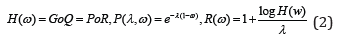
where P(ω) is the pgf of the Poisson distribution and R(ω) is the pgf of positive discrete rv with R (0) = 0.
Important class of the infinitely divisible distributions on Z+ are those which are selfdecomposable [3]. Let us recall that discrete random variable X Z+ ∈ .
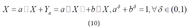
with the pgf G(ω) is called self-decomposable if it can be written as a sum of two independent variables [3]
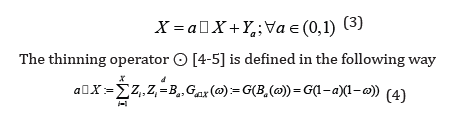
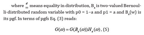
where Ha(ω) is the pgf of the rv Ya. It can be shown that the function Ha(ω) is absolutely monotone and infinitely divisible [3]. Obviously if G1(ω) and G2(ω) are self-decomposable pgfs then their product G1(ω)G2(ω) is also self-decomposable pgf. More general definitions of thinning operators were given in [6,7].
The importance of the thinning operation (4) for the rvs with finite mean is explained by the following theorem.
Theorem 1. Let Q(ω) be a pgf of the rv X such that EX = Q(1)(1) < ∞ and with scaled factorial moments Fj of order j

Then the rv Y = a ⊙ X with the pgf G(w) = Qa⊙X(w) has identical
scaled factorial moments as X.
Proof.

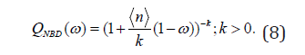
Example 1. Consider rv X with 〈n〉 := ΕX < ∞ which has the negative binomial distribution (NBD) with the pgf
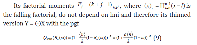
has not only the same scaled factorial moments as the rv X but is
also form-invariant w.r.t. scaling 〈n〉 →a n .
Returning back to the self-decomposable distributions we note
that there is only one distribution, discrete stable distribution (DSD),
for which the infinitely divisible component Ya is also self-decomposable
The canonical form (2) of its pgf reads

Where P(λ,ω) and S(λ,ω) the pgfs of Poisson and [8-10], respectively.
Let us note that there is a wide class of self-decomposable pgfs which similarly to Poisson (2), Bernouily (5), negative binomial (8) and discrete stable distributions (11) depend explicitly on the argument 1−ω , i.e., allow expansion of the type

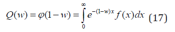
This category comprises also some less frequently used ones like the Mittag-Leffler Huillet & Martinez [10,9] distributions. Rather general construction of such pgfs is given in Klebanov [7]. More precisely, let ϕ(s) be the Laplace transform of a positive random variable X. Then

is a probability generating function.
The change of variable ω = (1− a) + az in (13) gives us

In other words, application of the thinning operator ω →1− a + az is equivalent to the scale change from 1 to a in the case of a ∈ (0,1). We can apply the thinning operator to arbitrary positive integer random variable but for the case of 0 < a < 1. However, ϕ(as) remains to be Laplace transform for any positive a. Naturally, we came to the problem: Describe all probability generating functions Q(ω) such that Q(1− a + aω) is again the pgf for all a > 0. The solution is given by the following result.
Theorem 2. Let Q(ω) be a probability generating function. Q(1− a + aω) is the pgf for all a > 0 if and only if there exists a Laplace transform of a positive random variable ϕ(s) such that the representation (13) holds.
Proof. Without loss of generality, we may consider the case a > 1.
1. Suppose that ϕ(s) is Laplace transform of a distribution function
and Q(ω) =ϕ (1−ω) is probability generating function. However,
ϕ(as) with arbitrary a > 0 is Laplace transform as well. According
to the result from [7] mentioned above, Q(a(1−ω)) = Q(1− a + aω) is
probability generating function for any a > 0.
2. Suppose that Q(1− a + aω) is probability generating function
for any a > 0. Define ϕ (s) = Q(1− s) . It is necessary to proof that
ϕ (s) is Laplace transform of a distribution function or, equivalently,
that it is absolutely monotone function. In other words, we have
to proof that


Because Q(1− a + aω) is probability generating function for any a > 0 the terms akQ(k) (1− a + aω) are non-negative for all 0 < w < 1 and all positive a. It proves absolutely monotones of ϕ(s). Corollary 1. Let P(N = n) = pn = Q(n)(0)/n!,n ∈ Z+ be a pmf of random variable N with the pgf Q(w) such that

Let us note that if pgf Q(w) has the representation (17) then for any b ∈ (0,1] the function Q(bw)/Q(b) is pgf and has the same representation with corresponding function fb(x). Namely,

It is also worth mentioning that the rv Y ∈ Z+ with the pgf Q(w)
satisfying Eq. (17) can be also interpreted as Poisson–distributed random
variable whose mean EY = X fluctuates according to the probability
density f(x) or, equivalently, as a mixture of the Poisson pgfs P(x,w)
= e−x(1−w) with the mixture weight f(x). Let us give few examples. Example
2. Consider pgf of the Hermite distribution [2]  describing sum of two independent random variables X1, X2 having
pgf
describing sum of two independent random variables X1, X2 having
pgf  and
and  correspondingly. Values of X1 are concentrated
on n = 0,1,2,3..., of X2 on even values only n = 0,2,4,6.... Hermite
distribution is infinitely divisible. Its pmf satisfies recursion
relation
correspondingly. Values of X1 are concentrated
on n = 0,1,2,3..., of X2 on even values only n = 0,2,4,6.... Hermite
distribution is infinitely divisible. Its pmf satisfies recursion
relation 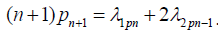 . For λ2 = 0 the recursion simplifies to
  and pgf Q(w) can be obtained from Eq. (13) with
  . However, for λ2 = 06 the density f(x) does not exist. On the
opposite side is the notoriously known example of the negative binomial
distribution with the pgf (8) which can be obtained from Eq. (13)
taking for f(x) the gamma distribution density
. However, for λ2 = 06 the density f(x) does not exist. On the
opposite side is the notoriously known example of the negative binomial
distribution with the pgf (8) which can be obtained from Eq. (13)
taking for f(x) the gamma distribution density  with β = (1− q) / q . Example 3. Let’s compare the pgf (11) of discrete
stable distribution with the Laplace integral [11].
with β = (1− q) / q . Example 3. Let’s compare the pgf (11) of discrete
stable distribution with the Laplace integral [11].
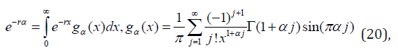
where gα(x) is the probability density function of the one-sided continuous stable distribution. Exact and explicit expressions for gα(x), for all α = l/k < 1, with k and l positive integers can be found in Penson & Gorska [12]. The substitutions γ = α and r = λ−γ (1 − w) in Eq. (20) enable us to express the pgf (11) as the Laplace transform (17) of the function.
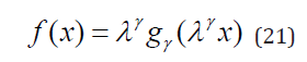
Hence the pmf of the discrete stable distribution satisfies the one step recurrence relation (n + 1) pn+1 = g(n)pn with g(n) given by Eq. (18) and f(x) by Eq. (21). It is worth mentioning that since a closed-form expression for pn using elementary functions is unknown the proof of this relation by the other methods is almost impossible.
Example 4. Consider random variable 1 Y = d = X + where Y ∈ N has Sibuya distribution. Then the rv X ∈ Z+ has shifted Sibuya distribution which is self-decomposable [13] and therefore also infinitely divisible [3]. Its pgf can be expressed via Eq. (17).

where Γ(a,x) is the incomplete gamma function with Γ(a,0) = Γ(a).
From Eq. (18) we obtain
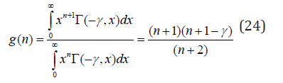
It is worth mentioning that the r-th absolute moment of the probability density function f(x) (23)
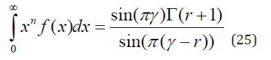
diverges for r > γ. This well-known property of the continuous heavy-tailed distributions is also shared by the family of discrete distribution represented by the Sibuya distribution. In the latter case the mean and higher moments hnri = Q(r) (w = 1), r ≥ 1 do not exist. One may naively expect that in this case also the Shannon entropy S = − Pn pn logpn of these distributions diverges. However, this is not the case. The∃ entropy S is finite either if or if r > 0 such that [14]. The following theorem establishes the condition when hnri < ∞, 0 < r < 1. Theorem 3. Integer-valued non-negative random variable Z with probability generating function Q(w) has finite r-th absolute moment (0 < r < a < 1) iff

Proof. For continuous non-negative random variable X with Laplace transform ϕ(u) = Ee−uX its r-th absolute moment 1 can be calculated using identity

Similarly, for the integer-valued non-negative random variable Z with Laplace transform ϕ (u) = Q(e−u) we have

Example 5. Consider N extended objects–particles each of the
same unit volume v0 = 1. Particles are incompressible and densely
packed occupying the total volume V = N in three-dimensional space.
If N is the Sibuya-distributed rv with the pgf S(γ,w) (11) then the integral
(26) and hence the corresponding moments ENr are finite only
for 0 < r < γ < 1. Consequently, the mean EV of the fluctuating volume
V d= N is nonexistent. However, for γ > 1/2 the mean value of the
enclosing surface as d well as of the linear extension, where
 means proportionality in distribution, of the 3d–space occupied by
particles are finite. Moreover for 1/2 ≥ γ > 1/3 ES does not exist but
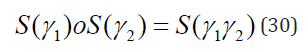
ER < ∞. Similarly, to the pgfs of Bernoulli and geometric distributions
Sibuya pgfs form a commutative semi-group under the operation of
compounding
means proportionality in distribution, of the 3d–space occupied by
particles are finite. Moreover for 1/2 ≥ γ > 1/3 ES does not exist but
ER < ∞. Similarly, to the pgfs of Bernoulli and geometric distributions
Sibuya pgfs form a commutative semi-group under the operation of
compounding
The following theorem establishes the additional similarity with Bernoulli distribution. Theorem 4. [15] Let Q(w) be the self-decomposable pgf of the random variable X on Z+ and S(γ,w) the pgf of Sibuya distribution. Then ∀γ ∈ (0,1) the function G(w) = QoS(γ) is also a self-decomposible pgf on Z+. Proof. We need to prove that ∀a the function
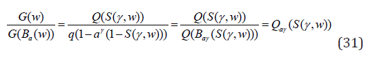
is also the pgf. This is true since Qαγ(S(w)) is a compound pgf ∀a ∈ (0,1). Remark 1. Obviously, sum of n independent self-decomposable rvs X1+...Xn is also self decomposable. The non-trivial character of the above theorem consists in the statement that this remains true also for the sum iid self-decompolsable rvs when n fluctuates according to the Sibuya distribution. Remark 2. Note that the thinned version of the Sibuya pgf appearing in Eq. 31
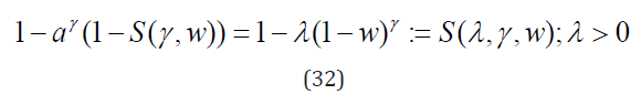
is the pgf of the scaled Sibuya distribution [13]. The latter is known to be infinitely divisible if and only if λ ≤ 1 − γ and self-decomposable if and only if λ ≤ (1 − γ)/(1 + γ) [13]. In this case, as follows from the Theorem 4, the pgf S(λ,γ)oS(α) is also self-decomposable. Corollary 2. Every Sibuya-distributed random variable X1 with parameter γ1 can be decomposed into the sum of two rvs X1 = X2 +Y, where X2 has the Sibuya distribution with parameter γ2 < γ1 and Y is self-decomposable. Proof. Let Q(w) be the pgf of the rv Y and γ1 = αγ2,0 < α < 1. Then

where S0(α, w) is the pgf of the shifted Sibuya distribution (22). The latter is self-decomposable [13] and so we can apply the Theorem 4 to obtain the needed result. Example 6. Skipping the trivial case of the discrete stable distribution (11) which is self-decomposable by construction let us consider the negative binomial distribution with parameter k = 1, so called geometric distribution, with the pgf Q(w) = (1+λ (1− w))−1 , cf. Eq. (8). Then

is the pgf of Mittag-Leffler distribution. Since Q(w) is self-decomposable decomposable it is also G(w). The random variable 1 Y d= X + with the pgf wG(w) where X has the pgf given by Eq. (35) with and λ = 1 describes the number of trials until the first return to the origin in one-dimensional symmetric random walk on the lattice Feller (1957).
Birth-And-Death Process
Let us consider continuous-time birth-and-death (B-D) process [1,16] consisting of random events of the same kind – e.g. creations and disintegrations of particles, populations of interacting species with indistinguishable members, queueing networks (interconnected queues) etc. The system represents a continuous-time Markov chain with a discrete state space n ∈ N which changes only through transitions from states to their nearest neighbors n → n ± 1. It is described by stochastic process {X(t) : t ≥ 0}

with transition probabilities Pi,j(t) satisfying Chapman-Kolmogorov equation

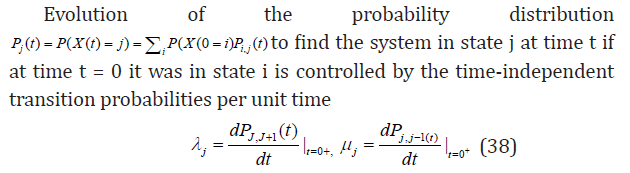
and satisfies differential-difference equation
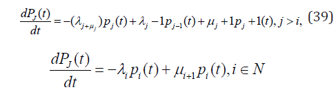
The last equation in (39) reflects the initial condition pj(0) = δij. One of the commonly used models specifying functional dependence of the transitional probabilities λj and μj on j considers j → j ± 1 transition as resulting from several underlying microscopic (particle-level) processes k → k ± 1, k = 0,...,j with the elementary transition probabilities αk and βk, respectively. Thus one particle is born or dies with the elementary probability per unit of time α0 or β0j, one particle can split into two particles with the rate α1j, two particles can fuse into a single particle with the rate β1j(j − 1), etc. The relations between the transitional probabilities λj and μj and elementary ones are given by the following formulas

For application of this approach to multiparticle production in high energy physics see e.g. (Biyajima, et al. [17,18]).
Stationary B-D Equations
It is well known that for large t solution of the B-D Eq. (39) can be well approximated by the limiting probabilities pj = limt→∞ pj(t) [1,16] which solve the Eq. (39) with dpj(t)/dt = 0. The latter is in this case transformed into two functional equations for one unknown function F(j)
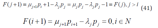
Solution of the first equation F(j+1) = F(j) is fixed to zero by the second equation F(i + 1) = 0. Consequently

We have thus proven the following theorem.
Theorem 5. The unique solution of Eqs. (42) with λj and μj given
by Eq. (40) reads:
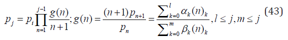
where pi is the first non-zero value of the positive sequence defining the pmf pj, i.e. mini≥0 pi > 0 and hence satisfying g(i) > 0 and g(i − 1) ≤ 0. Remark 3. Class of discrete distributions on Z+ satisfying the recursion formula (43) is substantially wider then usually discussed Kotz or Ord family of distributions or their generalizations Norman [19,20]. It is also worth nothing the similarity between Eq. (43) and pgfs satisfying Eq. (13). However, not every pgf satisfying Eq. (13) has its g(n)-function so simple that it can be written as in Eq. (43). To illustrate this point let us give two examples which are related to Sibuya-like distributions. The first is the thinned version of the shifted Sibuya distribution (22) with the pgf S0(Ba(w)). It is self-decomposable and so it can be expressed as the Laplace integral (17). Using Eq. (18) we can calculate its g–function to obtain
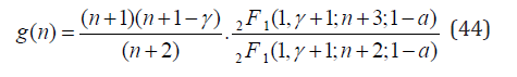
where 2F1(a1, a2;b1;z) is the Gauss hypergeometrical function. Obviously only for a = 1 the function g(n) can be expressed as a ratio of two polynomials in n. Another example is the pgf of the discrete stable distribution (11). Although its function f(x) does exist, see Eq. 21, its g(n)
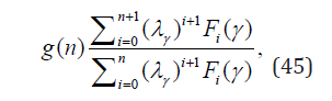
where the functions Fi(γ) are some polynomials in γ satisfying Fi(1) = 0,i > 0 with F0 = 1, it does not allow to be written in the form of Eq. (43). Corollary 3. The pmf (43) is the generalized hypergeometric probability distributions Norman with the pgf:

where ℓFm(a,b,z) represents the generalized hypergeometric function with series expansion

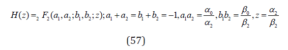
The constants a1,...,aℓ and b1,...,bm in Eq. (47) are some rational functions of α1,...,αℓ and β1,...,βm and z = αℓ/βm where αℓ and βm are the last non-zero transition amplitudes. Proof. Using Eq. (43) together with the identity

The last equality with 1/H(z) = pjz−jj! follows from the condition Q(1) = 1. Thus the pgf (48) corresponds to the power series distribution with the function H(z) which which is of the type of Eq. (47). Remark 4. Note the certain arbitrariness when associating the coefficients ai and bi with αi and βi, respectively. This is due to the permutation symmetry of the generalized hypergeometric function (47) w.r.t. its arguments ai and bi separately. Example 7. Consider Eq. (43) with ℓ = 1, j = 0, i.e. the case with the all coefficients α0, α1, β0, β1 positive. Then
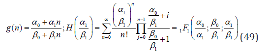
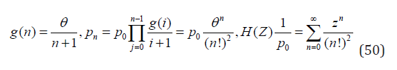
where 1F1(a;b;z) is Kummer’s (confluent hypergeometric) function. Neglecting in g(n) of Eq. (49) α1 and setting β0 = β1 with z = α0/β1 = θ yields the pmf of the Conway-Maxwell-Poisson (CMP) distribution with parameter r = 2 et al. (2005)
Expression for the scaled factorial moments (6) of this pmf obtained in Daly & Gaunt (2016) reads

It is worth mentioning that the pmf (50) has appeared in (Ko, et al. [21]) as a stationary solution of the kinetic master equation describing the production of charged particles which are created or destroyed only in pairs due to the conservation of their charge. On the other hand neglecting in g(n) of Eq. (49) the constant β1 we obtain the NBD

Example 8. Consider now more general case of Eq. (43) with ℓ = 2, j = 0

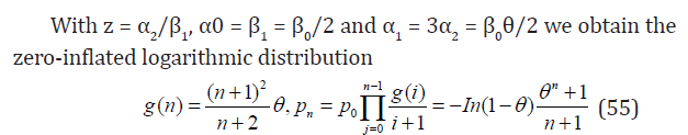
On the other hand, the logarithmic distribution can be reconstructed from

And similarly to the above case for the geometric distribution with g(n) = (n + 1) θ the only non-zero coefficients are α1 = 2β1θ,α2 = β1θ. Example 9. While the NBD (53) is frequently used in different areas of science e.g. in medicine [22,19] biology or in particle physics (Biyajima, et al. [17]); [23,24], the pmf obtained from Eq. (43) with non-zero α0, α2, β0, β2 and thus with the pgf Eq. (46) where
is seldom. Nevertheless, as shown in [18] it is important when describing the data with a secondary maximum (bump).
Generalized Sibuya Distribution
The Sibuya Distribution with The Probability Mass Function

first appeared in [8]. The generalized Sibuya distribution with parameters ν ≥ 0 and 0 < γ < ν +1 has been introduced in [25] as the distribution of the number N of trials until series of the Bernoulli trials with the varying success probability γ/(ν + n − 1) and thus having the probability mass function

One connection of the generalized Sibuya distribution with the classical Sibuya variable N is through the probability of the excess P(N − m = n|N > m), which has the generalized Sibuya distribution with ν = m. This extends to the generalized Sibuya variable N for which P(N −m = n|N > m) has also the generalized Sibuya distribution with ν + m as its parameter. Writing the pmf (59) as
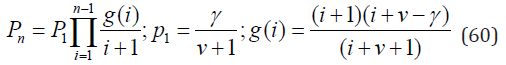
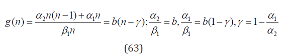
we can see that function g(i) of the generalized Sibuya distribution is a special case of Eq. (54) with β2 = 0 and thus solves the stationary B-D equations (42). The corresponding non-zero coefficients are

Moreover, for ν = 0 we have p1 = γ and Eq. (60) reduces to the pmf of Sibuya distribution (11). The pgf of the generalized Sibuya distribution calculated from Eq. (60) reads
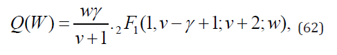
where 2F1(a1,a2;b1;z) is the Gauss hypergeometric function.
Extended Sibuya Distribution
Consider now Eq. (43) with ℓ = 2,j = 1 and hence with the function g(n) given by Eq. (54) with α0 = β0 = 0
Using Corollary 3 it is easy to verify that the corresponding pgf
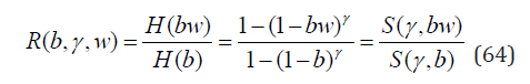
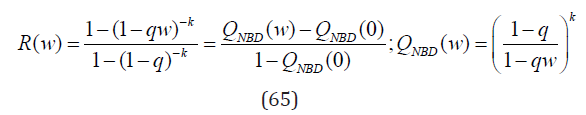
represents yet another generalization of the Sibuya pgf S(γ,w). For γ = −k < 0 and fixed b = q the pgf (64) coincides with the NBD pgf (8) truncated at zero
For γ → 0, i.e. when α2 → α1, the pgf (64) approaches the logarithmic distribution

and for γ → 1 it converges to distribution with the pmf pn = δ1n. Let us note that the pgf (64) was already mentioned in Letac (2019) (see Eq.(6) therein) as the natural exponential family extension of the Sibuya distribution. Since no name was given to it nor its relation with the other known distributions was discussed we take a liberty and call it the pgf of extended Sibuya distribution stressing its smooth transition in γ to the pgfs of several fundamental discrete distributions. Let us now study the factorial moments
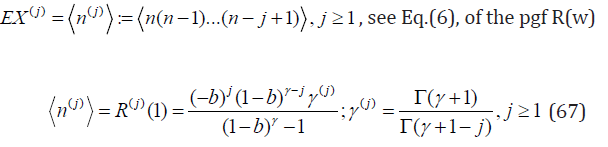
When approaching the Sibuya distribution, i.e. for b → 1− we obtain expected results

For the second scaled factorial moment F2, cf. Eq. (6) we have
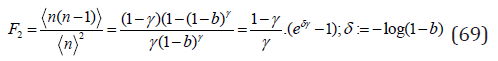
Ignoring the region with γ < 0 which corresponds to the zero- truncated NBD let us analyze the behavior of
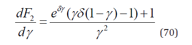
For γ → 0, i.e. for the logarithmic distribution, F2 has a minimum at δ = 2. Further up, in the region (γ > 0,δ > 2), the extreme of F2(γ) moves along the trajectory dF2/dγ|γ0 = 0 or equivalently ψ(γ0,δ) = 0, where ψ (γ ,δ ) = (eγδ (γδ (1−γ ) −1) +1. While F2(γ) increases for 0 < γ < γ0 it decreases for γ0 < γ < 1. When approaching the singularity at b = 1 the second scaled factorial moment F2 and hence also its maximum goes to infinity. Let us add that the same maxima appear also in the higher scaled factorial moments Fj,j > 2.
The Shifted Variants of Extended and Generalized Sibuya Distributions
Consider random variable Y d= X + 1 where Y ∈ N has either extended or generalized Sibuya distribution. Then the rv X ∈ Z+ has shifted extended or generalized Sibuya distribution, respectively. The case when Y has ordinary Sibuya distribution was already discussed in Example 4. Note that contrary to the original extended or generalized Sibuya distributions their shifted variants are now defined on Z+ and so they may be self-decomposable.
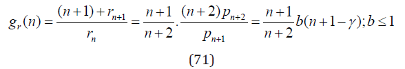
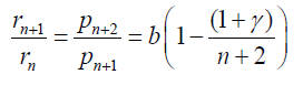
The Shifted Extended Sibuya Distribution: If pn and R(b,γ,w) are the pmf the pgf of the extended Sibuya distribution (63), respectively, then rn = pn+1 and R0(b,γ,w) = R(b,γ,w)/w, cf. Eq. (22), are the pmf and the pgf of the shifted extended Sibuya distribution. Corresponding function g(n) thus reads
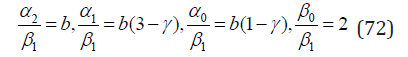
cf. Eq. (24). The elementary transition amplitudes (43) derived from Eq. (71) are
Theorem 6. The shifted extended Sibuya distribution is self-decomposable. Proof. Following [13] we use Lemma 1. [26] A strictly decreasing pmf rn,n = 0,1,2,... such that
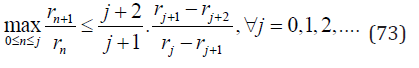
is discrete self-decomposable. In our case the sequence
is strictly decreasing and therefore the left-hand side of Eq. (73)

Now we need to prove that R(b,j) ≥ 1. It is easy to verify that R(b,j) is decreasing function with respect to b for each fixed j. Therefore, its minimum is attained at point b = 1 where
Hence Eq. (73) is satisfied and the shifted extended Sibuya distribution is indeed self-decomposable and thus also infinitely divisible [3]. For b < 1 the Theorem 1 tells us that the scaled factorial moments of the shifted extended Sibuya distribution with the pgf R0(b,γ,w) and of its thinned version R0(b,γ,1− a + aw) are the same. Moreover, since R0(b,γ,w) = S0(γ,bw)/S0(γ,b), see Eq. (64), it is easy to check using Eq. 19 with f(x) given by Eq. (23) that the pgf of the shifted extended Sibuya distribution satisfies the Theorem 2 and hence the scaling variable a can be any positive number.
The Shifted Generalized Sibuya Distribution: If pn is the pmf of the generalized Sibuya distribution (59) then rn = pn+1 is the pmf of the shifted generalized Sibuya distribution with the g-function

and hence
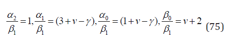
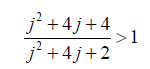
Interestingly, the only difference between the coefficients of the original (61) and the shifted distribution (75) consists in replacement ν → ν + 1. To check the self-decomposability, we once again use the Lemma 1 to find that

is strictly decreasing. Therefore the l.h.s. of the Eq. (73) gives:
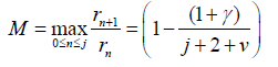
Using Eq. (74) we rewrite the r.h.s. of the Eq. (73) as

Dividing now the r.h.s. of the Eq. (73) by its l.h.s. and neglecting terms O (j−3) we observe that there always ∃j0 > 0 such that ∀j ≥ j0 the ratio
where in that last equation we have used the inequality 0 < γ < ν +1. Thus, contrary to the previous case the shifted generalized Sibuya distribution is not self-decomposable.
Beyond The Sibuya Distribution
Let us consider the following four-parameter generalization of the Sibuya pgf

In [7] it was shown that Eq. (76) represents a probability generating function in the case of γ = 1/m, k = m, b = 1 where m, ℓ ∈ N. It is not difficult to prove this statement remains true for the case of positive integer k ≤ m and b ∈ (0,1]. For the case of k = ℓ = 1 the function Q(w) coincides with probability generating function R(w) of the extended Sibuya distribution (64). For the case of k = 1 the pgf Eq. (76) represents the sum of ℓ extended Sibuya– distributed random variables. In particular, for ℓ = 2, the function g(n) is easily calculable

Let us note that for γ ≥ 1/2 the function (77) is positive and for n ≥ 2 it is close to linear function of n g(n) ≈ a1(γ)(n + a2(γ)). In particular for γ = 1/2 it coincides with the extended Sibuya distribution (63). On the other hand, for k = ℓ = 2, m ≥ 2 the ratio g(n) (43) takes the form

Most simple case is m = 2 with  which is positive for
n ≥ 2. The pmf then reads.
which is positive for
n ≥ 2. The pmf then reads.
The Extended Sibuya as Progeny
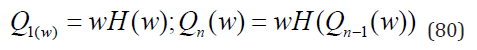
Consider branching process (Zn)∞N≥0 governed by the pmf pk, k ∈ Z+ [1,27]. Markov property of the process determines how the direct descendants of the nth generation form the (n+1)st generation. If Zn is the size of the nth generation and Hn(w) is its pgf then rv Yn = 1 + Z1 + ... + Zn with the pgf Qn(w) represents the total number of descendants up to the nth generation including the ancestor (zero generation). By assumption and therefore
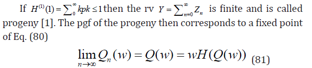
By inverting the last equation we can express H(w) in terms of Q(w)
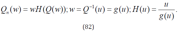
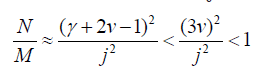
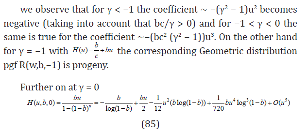
Note that although such inversion is in principle always possible the rv Y is the progeny only when all the expansion coefficients of the function H(u) in powers of u are positive. In particular, for the case of Sibuya pgf (11) Eq. (82) with Q(w) = S(γ,w) the progeny was shown to exists only for 1/2 ≤γ < 1[28-30]. For the extended Sibuya distribution Eq. (82) with Q(w) = R(w) yields
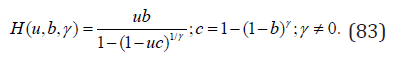
Expanding H(u,b,γ) in powers of u

it is now coefficient ∼ log3(1 − b)u4 which is negative. Finally for γ > 0 substitution t = bw → w in Eq. (64) yields the pgf of Sibuya distribution (11) S(t) multiplied by positive factor 1/(1 − (1 − b)γ) and hence with the identical signs of all expansion coefficients. Therefore


The goal of this article was to discuss the properties of Sibuya-like random variables related to their scaling and birth-death processes. We have shown that their pmf satisfy a one-step recurrence relation g(n) = (n+1)pn-1/pn with some of them representing the stationary solutions of the birth-death equations and most of them being self-decomposable. In addition to already known Sibuya-like distribution (shifted Sibuya, generalized Sibuya, disctere stable) we have found a new one - extended Sibuya distribution. The latter is very similar to ordinary Sibuya distribution having the same bounds of its validity as a progeny in branching process.
The work of Lev B. Klebanov was partially supported by Grant 19- 28231X GA CR.ˇ Michal Sumbera is partially supported by the grants LTT17018 and LTT18002 of theˇ Ministry of Education of the Czech Republic.


