Rational Control of Global Warming Dynamics Via the CO₂ Level, Emission Reductions and Forestry Expansion Volume 47- Issue 3

Peter Lohmander*

• Optimal Solutions, Hoppets Grand 6, 903 34 Umea, Sweden

Received: November 09, 2022;   Published: December 05, 2022

*Corresponding author: Peter Lohmander, Optimal Solutions, Hoppets Grand 6, 903 34 Umea, Sweden

DOI: 10.26717/BJSTR.2022.47.007501

Abstract PDF

First, the observed CO₂ level in the atmosphere, recorded by NOAA [1] at the Mauna Loa observatory, and the global industrial CO₂ emissions, reported by EDGAR [2], European Commission, are investigated, from 1990 until 2021. Then, a differential equation model is developed, based on two hypotheses, that explains how these time series interact. The hypotheses of the explaining model are tested with regression analysis, and it is demonstrated that no hypothesis can be rejected on statistical grounds. The parameters of the CO₂ concentration model are determined with high t-values and low p-values. The model is used to determine the time path of the CO₂ concentration of the natural system without industrial emissions, for arbitrary initial conditions. This system has a unique and stable equilibrium at 262 ppm. With constant industrial emissions, the equilibrium is found at a higher level, which is shown with an explicit equation. Comparative statics analysis shows how the equilibrium is affected by alternative parameter adjustments. An extended version of the natural differential equation, with a forcing function, representing the time paths of industrial emissions, is developed. The industrial emissions are modeled as a quadratic function of time. The general function of the time path of the CO₂ concentration of the natural system under the influence of industrial emissions, is determined for arbitrary initial conditions and parameters of the industrial emission function.

The CO₂ time path function is analytically verified. Then, it is also empirically tested and found to be able to reproduce the historical CO₂ observations with high precision. Then, the time paths of the future CO₂ concentrations are calculated, for six alternative levels of change of the industrial emissions, from -1.5 Gt/year to +1.0 Gt/ year, from the year 2022 until 2100. These results are presented as a function and as graphs. The net CO₂ emissions can also be reduced over time, if forestry is gradually intensified. The rational intensity of this investment process is determined, taking the time path of the CO₂ level into consideration, during an arbitrary time interval. An explicit function for the optimal forestry intensification level, based on all CO₂ time path function parameters, the marginal cost of the CO₂ concentration, time interval parameters, rate of interest and different cost function parameters, is derived and presented.

Keywords: Global Warming; Co₂ Dynamics; Co₂ Predictions; Emission Control Optimization; Optimized Forestry

Rational management to avoid global warming is complicated. International cooperation and rational decisions are obviously necessary in this process. Our world however presently faces several severe conflicts and sources of instability. The problem areas are connected and interdependent in several ways. We observe large scale geopolitical tensions with local and global disturbances such as the covid-19 pandemic, the war between Russia and Ukraine, large streams of refugees, global warming and expanding wild fires. Europe, presently dependent on large imports of Russian fossil fuels such as oil, gas and coal, is intensively investigating new ways to simultaneously increase energy independence and to reduce future global warming. The technology options of energy systems and environmental problems rapidly develop. International control, such as global taxes on CO₂, are discussed and environmental initiatives of many kinds, such as investments in solar power and wind power, are made in many regions. Combined heat and power, CHP, based on combinations of waste and forest fuels, expands in the Nordic countries. New ways to continuously and sustainably manage the global forest resources have been developed that not only optimize profits but also contribute to the CO₂ management problem. Furthermore, carbon capture and storage can make several kinds of energy systems sustainable. Global warming, and the CO₂ concentration, are fundamentally linked via the greenhouse effect of the gas CO₂.

A study of the past development of the CO₂ concentration in the atmosphere, included in this paper, is very important to get a perspective on the dramatic development. The key to rational future climate management, is to understand the options to control the future CO₂ concentration via different methods. Brown, et al. [3] presented several ways to manage forests to mitigate CO₂ emissions. Some of these methods were to reduce the speed of deforestation, to change harvesting regimes, to protect forests from disturbances, to increase the area and density of forests, to increase substitution, for instance to let forest fuels and forest products replace fossil-fuels and products based on them. They estimated the sizes of the areas where these methods could be used. Then, they derived the atmospheric CO₂ effects of these forestry methods and estimated that these were equivalent to 11-15% of the fossil fuel emissions. The costs of the different methods were also estimated in $US per Mg C. The article by Brown, et al. [3] certainly is impressive. It handles several relevant questions and gives concrete solutions. Later, several other authors continued to investigate these problems. Favero, et al. [4] essentially came to similar conclusions, for instance that expanded use of wood for bioenergy will result in net carbon benefits. They also touch upon the public debate, which contains several aspects on the roles of forests. Forster, et al. [5] investigate the same problems, but also build the analysis on real data connected to the UK national planting strategy.

They find that commercial afforestation can deliver effective green house gas mitigation that is robust to future decarbonization pathways and wood uses. Holmgren [6] focuses on similar topics but builds the analysis using forest sector data from Sweden. He is very critical towards the current public forest debate and the EU-level forest policy development. These mostly advocate reduced harvesting in order to increase the carbon contents of the forests. However, Holmgren [6] finds that “no climate advantage was found for no-harvest or reduced-harvest scenarios, despite commonly expressed views in the debate”. The conclusions by Holmgren [6] are rational, when we consider the articles by Brown, et al. [3-5]. Similar conclusions can be found also in other studies. Lohmander [7] concludes: “If the relative weight of the utility of the climate increases, the optimal area of natural forests that should be transformed to managed continuous cover forests increases.” Lohmander [8] writes that if the area of active forest management increases, the area covered by forests in dynamic equilibria with net CO₂ absorption close to zero, decreases. He also formally proves that: “If it is considered more important to avoid global warming, then we should increase the use of forest energy inputs and decrease the use of fossil energy inputs in the combined heat and power industry. This was proved with a general function model that was not dependent on particular numerical parameter values.

The derived results contradict the common opinion that the best way to use the forest with consideration of global warming, is to maximize the stock level in the forest, and if possible, to completely stop harvesting. A compact and fundamental theory of the CO₂ level in the atmosphere, under the influence of changing CO₂ emissions, was developed as a first order linear differential equation with a forcing function, describing industrial emissions, by Lohmander [9]. The general mathematical methods of such analyses are found in Braun [10]. Observations of the CO₂ level at the Mauna Loa CO₂ observatory, NOAA [1], and official statistics of global CO₂ emissions, from EDGAR [2], the Joint Research Centre at the European Commission, were used to estimate all parameters of the forced CO₂ differential equation. The estimated differential equation was used to reproduce the time path of the CO₂ data from Mauna Loa, from year 1990 to 2018, with very small errors. With that differential equation model, the global CO₂ level, without emissions, has a stable equilibrium at 280 ppm. This value has earlier been reported by IPCC, in Solomon, et al. [11], as the pre-industrial CO₂ level. Reduced global industrial emissions of CO₂ can solve a large part of the global warming problem, as reported by Lohmander [9], and intensified forestry can absorb considerable amounts of CO₂, along the lines found in many of the articles discussed above.

As mentioned by Holmgren [6], the current forest debate is however often skeptical towards intensified forest production, even if that can solve parts of the climate problems. A main reason for this attitude frequently is the implicit assumption that intensified forest production has to be based on clearcutting (simultaneous harvesting of all trees) and other environmentally disturbing forestry methods. In many countries, commercial forestry based on clearcuts is and has been the dominating forest management method for a long time. Recently, however, new research in the area of forest production has made it possible to understand and optimize forest management based on continuous cover forestry. (With such methods, the forest always contains trees of different sizes. The largest trees are periodically harvested and the smaller trees are left in the forest to continue to grow.) Hatami, et al. [12,13] are two studies where the growth functions for individual trees have been developed. With such functions, it is possible to mathematically develop economically and environmentally rational continuous cover forestry decision rules. These rules can also be optimized to handle the global warming problem. Our world is covered by large areas of primary (natural) forests that are almost not managed at all. They do not contribute very much to the net absorption of CO₂. (The reason is that the old trees sooner or later die, fall in storms or burn in fires. Then, the CO₂ stored in these trees is released to the atmosphere.)

Large parts of these natural forests may be transformed to continuous cover forests, which means that the net absorption of CO₂ increases so that the CO₂ level in the atmosphere can be further reduced. This transformation can be made without severely damaging the environmental conditions. We may define an optimization problem with two objectives with different weights in the objective function. These objectives can be the economic present value of profits and the utility of the climate. The optimal transformation of natural forests to managed continuous cover forests is then affected by the relative weights of the utility of the climate and of the present value of the profits. If the relative weight of the utility of the climate increases, the optimal area of natural forests that should be transformed to managed continuous cover forests increases. Several concrete results were reported in this area by Lohmander [7,8]. Forests, sensitive to fires, cover large parts of our planet. Rational protection of forests against fires, forest fire management, is a very important topic area. Global warming affects fires and fires affect global warming via CO₂ emissions. Forest fires cause severe problems in many countries. Forest fire areas in nine European countries were investigated by Lohmander [14] with respect to yearly averages, standard deviations and correlations between nations. In the region IFPS (Italy, France, Portugal and Spain), the average yearly burned area during the years 2010 to 2018 was 313.4 kha and in FGLNS (Finland, Germany, Latvia, Norway and Sweden) the corresponding area was only 7.6 kha.

The correlations between the regions are strictly negative and the correlations within the regions are strictly positive. Since forest fires usually do not occur in every country at the same time, there is a potential expected gain from international cooperation, where easily mobile firefighting resources such as water bombing airplanes are moved between nations. A general stochastic dynamic programming approach to adaptive moves of such resources was defined and suggested. It was demonstrated that the expected objective function value, the expected present value of total costs, is a strictly increasing function of the fire correlation between nations. Adaptive moves of mobile resources between the regions IFPS and FGLNS have the advantage of negative correlations between these regions. Some adaptive moves can also be motivated within the regions even with positive correlations, thanks to the low costs of short moves. The average relative burned areas have been studied by Lohmander [15], as a function of different conditions, in 29 countries. Detailed international statistics of forest fires, were used as empirical data. A multivariate fire area function with empirically very convincing statistical properties was defined, tested, and estimated. Future fire areas were predicted for 29 countries, conditional on three alternative levels of global warming. Global warming was predicted to make future forest fire problems more severe. A methodologically connected study, based on detailed empirical data from Czech Republic, was also published by Mohammadi, et al. [16].

The probabilities of long dry periods and strong winds are increasing functions of a warmer climate. Heat, dry conditions and strong winds increase the probabilities that fires start. Furthermore, if a fire starts, the stronger winds make the fires spread more rapidly and the destruction increases. Under the influence of global warming, we may expect more severe problems in forestry caused by wild fires. For all of these reasons, Lohmander [17] investigated and optimized the general principles of the combined forestry and wild fire management problem. In this process, we should integrate the infrastructure and the firefighting resources in the system as decision variables in the optimization problem. First, analytical methods were used to determine general results concerning how the optimal decisions are affected by increasing wind speed, and implicitly, increasing temperature. The total system was analyzed with one dimensional optimization. Then, different combinations of decisions were optimized and the importance of optimal coordination was demonstrated. Finally, a particular numerical version of the optimization problem was constructed and studied. The main results, under the influence of global warming, were the following: In order to improve the expected total results, we should reduce the stock level in the forests, increase the level of fuel treatment, increase the capacity of firefighting resources and increase the density of the road network. The total expected present value of all activities in a forest region are reduced even if optimal adjustments are made.

These results were derived via analytical optimization and comparative statics analysis. They have also been confirmed via a numerical nonlinear programming model where all decisions simultaneously were optimized.

In order to reduce the CO₂ emissions, it is important to be able to stop fires before they have become too large. The time to reach the fire strongly affects the size of the burned areas. For this reason, the distance between fire stations is an important decision variable, that should be optimized. This is studied by Lohmander [18]. He proved that the optimal distance is a function of several conditions that differ between regions and seasons. The optimal distance is a strictly decreasing function of the expected number of fires per area unit, a strictly increasing function of the speed of the fire engines, a strictly decreasing function of the parameters of the exponential fire cost function, and a strictly increasing function of the cost per fire station. Several of the connected principles and results were summarized and presented in Lohmander [19]. The present analysis is founded on ideas and results from several recent articles that have never before been treated in combination.

As a first step, the model and the results from Lohmander [9] are extended and updated, via an increased number of empirical observations, a more detailed statistical analysis and a more detailed dynamic analysis.

The analysis in this paper, “B”, is based on another method than Lohmander [9], “A”.

In the earlier study, A, the parameters of the CO₂ differential equation were calculated from a very small number of averages of empirical observations, via basic linear algebra. In the present study, B, however, a full statistical regression analysis was used to estimate the parameters of the corresponding differential equation. Hence, the number of observations is much higher in B than in A, where only period averages were used as simple data.

When we want to apply the CO₂ differential equation, in order to predict future values, and in particular to optimize emission reduction decisions and forestry expansion decisions, it is very important to know how well we can trust the estimated parameter values. With the statistical method used in the present study, B, we obtain and report standard errors and P-values of the estimated parameters of the CO₂ concentration differential equation. In the earlier study, A, no such results were calculated and reported, because the method applied in A could not give any such estimates. So, now, for the first time, we obtain important new information about the parameters that has earlier not existed. The present analysis, B, is based on longer time series of empirical data than A, since new data have become available over time. We are living in a world of global warming and every new piece of information is important. Hence, the new functions in B should be expected to be a more relevant and reliable than the functions in A. It will be seen that, with the function estimated in this study, B, the estimated equilibrium CO₂ value without industrial emissions, is 262 ppm, and not 280 ppm, as reported in the earlier study A.

Hence, “B” should give a new, more relevant, and more reliable, perspective on historical observations of CO₂ levels, compared to A. Alternative levels of industrial emission scenarios from 2022 to 2100 will be defined and the consequences for the time paths of the CO₂ concentration in the atmosphere will be determined. Furthermore, the optimal expansion of active forest management, under the influence of global warming, will be determined, in the form of an explicit function. This study, B, contains several central problems and analyses that are not at all discussed and/or handled in earlies studies, such as A. For instance, we will see how the level of change of the net CO₂ emissions should be dynamically optimized. This is done in high detail, via 35 equations. It is shown how this change depends on industrial emissions and expansion of forestry activities. It is shown that the optimal solution under the described assumptions gives a unique maximum to a defined multi objective function, and how the optimal solution depends on the properties of the utility function, in which the utility of the climate, transformed to the utility of the CO₂ level, and the different kinds of investment costs, are considered. The analysis leads to an explicit solution to the optimal decisions. This quite new result gives the optimal investment level in more productive and sustainable forestry as an explicit function of all of the parameters. Similar results have not been reported in earlier studies.

The empirical data used in this study contains the time series of the CO₂ level in the atmosphere, from NOAA [1], and the time series of industrial emissions of CO₂, from EDGAR [2]. These time series are found in the Appendix. In the Appendix, we also find some transformations of the data series, that are motivated by the mathematical and statistical analyses in this paper. The NOAA [1] data series contains one observation per year. The series in EDGAR [2] have longer time intervals between the observations. For this reason, linear interpolation is used to calculate estimated emission data between the reported observations. These interpolations can be investigated in the Appendix. The dramatic development of the CO₂ concentration in the atmosphere is illustrated in (Figures 1 & 2). Compare the differenced series and the connections to the industrial CO₂ emissions, as illustrated in (Figure 3). In (Figure 3), we see three graphs of time series, representing the time interval year 1990 until year 2120. They show the industrial CO₂ emissions to the atmosphere, the change of the CO₂ level in the atmosphere and the difference between these series. During the investigated period, the industrial CO₂ emissions are always larger than the increase of the CO₂ level in the atmosphere. Clearly, the CO₂ level in the at mosphere increases less than the industrial CO₂ emissions, which indicates that some part of the CO₂ in the atmosphere leaves the atmosphere, to be absorbed elsewhere. This will be investigated in detail, in the following analysis.

Figure 1.The CO₂ concentration in the atmosphere, in the unit ppm, according to the observations from the Mauna Loa observatory. Source: NOAA [1].

Figure 2.The CO₂ level in the atmosphere, in the unit Gt, according to the observations from the Mauna Loa observatory and variable transformations. Sources: NOAA [1,20].

Figure 3.The CO₂ emissions to the atmosphere, e_Gt, in the unit Gt, the change during one year of the CO₂ level in the atmosphere, delta_x_Gt, and the yearly change of the CO₂ level in the atmosphere reduced by the emissions, delta_(x-e) Gt, in the unit Gt. Sources: NOAA [1,2,20].

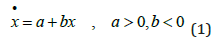
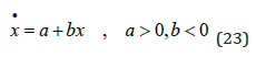
We start by modeling the “natural CO₂ system”, without “exogenous industrial CO₂ emissions”, as the differential equation (1). The CO₂ level in the atmosphere is x. The time derivative of x is marked with a dot, in the spirit of Newtonian notation. Natural emissions from the environment, including volcanos, are represented by the parameter a. Of course, a should be strictly positive. Compare equation (1). We assume that the natural environment, including the oceans, absorb some of the CO₂ in the atmosphere, and that this absorption is proportional to the CO₂ level in the atmosphere. This form of absorption law can be motivated, with simple physical arguments. For instance: We consider air temperature as fixed, which means that the velocity distribution of CO₂ molecules is held constant. Then, if we double the number of CO₂ molecules in the atmosphere, the number of molecules that touch the surface of the ocean per time unit, approximately also doubles. This makes it understandable that the absorption of CO₂ by the ocean is more or less proportional to the concentration of CO₂ in the atmosphere. Hence, the absorption parameter b should be strictly negative, which is also seen in equation (1).

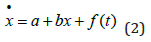
In the empirical data, the time derivative of x is also affected by f(t), which represents the total industrial emissions as a function of time.

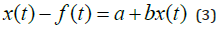
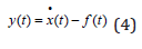
We may reformulate (2) to get (3) and (4).

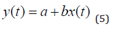
In regression analysis, we estimate y(t) as a function of the parameters a, b and the value of x(t). Compare (4) and (5) and the Appendix.

The results from the parameter estimations are found in (Tables 1 & 2).

Table 1. Estimated regression parameters when the unit of x(t) is Gt. y(t) and the time derivative of x(t), have the unit Gt/year. The parameters have five value figures in this table. All of the regression results and the data are found in the Appendix.

Table 2. Estimated regression parameters when the unit of x(t) is ppm. y(t) and the time derivative of x(t), have the unit ppm/year. The parameters have five value figures in this table. All of the regression information and the data are found in the Appendix.

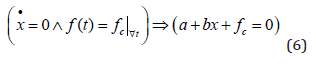
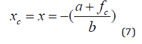
In case the industrial emissions would be constant and equal to f_c, then in CO₂ equilibrium, x_c, equation (6) is satisfied, which leads to (7).

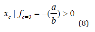
Without industrial emissions, the equilibrium is (8).

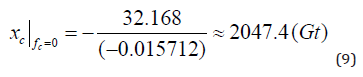
We can now use equation (8) to determine the equilibrium value of the natural system. When we use the unit Gt, as in (Table 1), we get the result in equation (9).

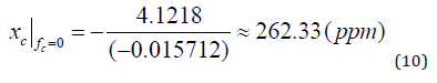
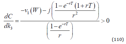
If we use the unit ppm, as in (Table 2), we get the result in equation (10).

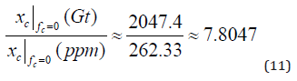
Following the principles by O Hara [20], the following transformation rules have been applied: 1 ppm (CO₂) can be transformed to 2.13*3.664=7.80432 Gt CO₂. 1 ppm by volume of atmosphere CO₂ =2.13 Gt C. 1 g C=0.083 mole CO₂ =3.664 g CO₂. Hence, we may change units, and go to the unit ppm from the unit Gt, if we divide the figure in Gt by 7.80432.

In equation (11), we find that the ratio is very close to the correct figure, also if we only use five value figures.

Comparative statics analysis of the CO₂ equilibrium with constant emissions:
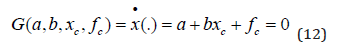
If the CO₂ level in the atmosphere is in equilibrium and the exogenous industrial emissions are constant over time, for instance zero, then equation (12) is satisfied.

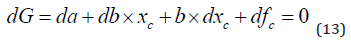
Total differentiation of the equilibrium condition gives (13).

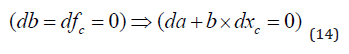
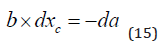
First, we study how the CO₂ equilibrium level in the atmosphere changes if the natural emissions increase. This is found in equation (14). Equation (15) follows.

As we see in (16), the equilibrium CO₂ level in the atmosphere is a strictly increasing function of the level of the natural emissions. The value of b, reported in (Tables 1 & 2), combined with equation (16), can be used to derive an explicit numerical value of the derivative.

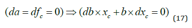
The effect of changes in the absorption coefficient b on the equilibrium CO₂ level in the atmosphere is studied in equations (17) and (18).

If b increases, the absorption decreases. As we see in (19), the CO₂ equilibrium level in the atmosphere is a strictly increasing function of b, which means that it is a strictly decreasing function of the natural absorption level.

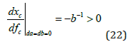
In equations (20) and (21), the effect of the exogenous industrial emission level is under analysis.

Equation (22) tells us that the equilibrium CO₂ level in the atmosphere is a strictly increasing function of the exogenous industrial emission level. The value of the derivative is identical to the value of the derivative (16).

Explicit dynamics analysis of the natural system
Now, we will derive the CO₂ level in the atmosphere as an explicit function of time, in case we have a natural system, (23), without any exogenous industrial emissions.

(23) can be written as (24).

First, we study the homogenous equation, (25) and try to find an explicit solution.

We assume that the homogenous solution, X_h(t) has the functional form found in (26). Z and λ are two parameters.

The time derivative of the homogenous solution is found in (27).

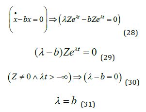
Equations (28) to (31) give the value of λ .

The homogenous solution is reported in (32). This now contains one parameter that has not yet been determined, namely Z . Considerable efforts will be used to determine this parameter as a function of other relevant parameters, in the later part of this paper.

Particular solution It is also necessary to determine the particular solution. We start with equation (33).

We assume that the particular solution is an arbitrary constant, as in (34).

As we see in (35), the time derivative of the particular solution is zero.

(33), (34) and (35) give (36) and (37).

(37) leads to the particular solution, namely equation (38).

The complete solution to the differential equation is the sum of the homogenous solution and the particular solution. Compare (39).

The explicit form of the solution to the natural system is found in (40).

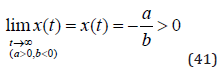
Since we already know that the value of b is strictly negative, it is clear that the homogenous solution (32) goes to zero as t goes to infinity. As a consequence, as we see in (41), the equilibrium is stable. Equation (40) also reveals that we have monotone convergence to the equilibrium. Furthermore, since the natural emission level is strictly positive, the equilibrium is strictly positive. Note that this equilibrium was also found in equation (8) and that the numerical values were derived in different units, in equations (9) and (10).

Explicit dynamics analysis of the natural system with added exogenous forcing
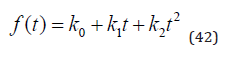
Now, we introduce exogenous (industrial) net emissions as an explicit function of time, in equation (42). This makes it possible to represent the future time path of alternative global CO₂ emissions as a quadratic function of time. Certainly, also other functional forms could be used. The polynomial is however a flexible tool with suitable properties for the relevant applications that will follow. We may also use the function to model alternative forestry expansion strategies, where intensified forestry can lead to increased absorption of CO₂.

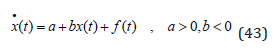
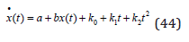
When (42) is added to the natural system differential function, we get (43).

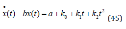
The explicit version of (43) is (44). This may also be transformed to (45).

From (45) we understand that the solution to the homogenous solution, (32), will be useful also when we solve (45).

>Determination of the Particular Solution

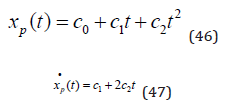
Now, we need a more complicated functional form of the particular solution than when we only had to deal with the natural system, without changing exogenous emissions, as in equation (34).
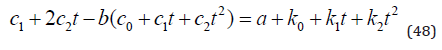
The time derivative of the particular solution is (47).

(45), (46) and (47) lead to (48). We have to determine the three parameters in the particular solution, found in (46), from equation (48).

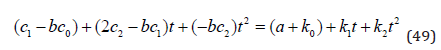
It is clear that (48) has to be satisfied for every possible value of t. In (49), the LHS and RHS expressions are written in a more convenient form.

We realize that the equation system found in (50) has to be satisfied. That system will hopefully be useful to derive the correct parameters of the particular solution (46).

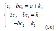
In (51), the equation system in (50) is represented in matrix format.

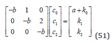
We find that the system has a structure that makes it possible to solve it with a sequence of substitutions. If that would not have been the case, we could have used other methods from matrix algebra. From row 3, we instantly get the value of c2. This is shown in (52).

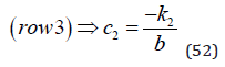
Then we move to row 2, which can be used to derive c₁ , using c₂ and some parameters. Compare equation (53).

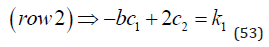
Equations (54), (55) and (56) lead to the value of c₁.

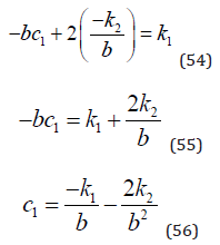
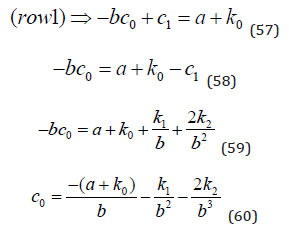
Finally, we can derive c0 via equations (57) to (60).

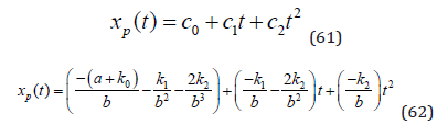
The particular solution (61) is found in explicit form in (62).

The CO₂ level in the atmosphere, (63), is the sum of the homogenous solution and the particular solution.

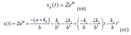
The homogenous solution is found in (64) and the CO₂ level in the atmosphere is shown in (65).

Clearly, before we move further and apply function (65), it is important to verify that the function is correct. We use the following procedure: First we derive the time derivative of (65), namely (66).

Then, we remember the original differential equation (67).

Equation (66) is defined from equation (68).

Equation (69) is defined from equation (67).

We denote the difference between the expressions (68) and (69) by (70). Then, we find that the difference is zero, which means that the expressions are equal, as in equation (70).

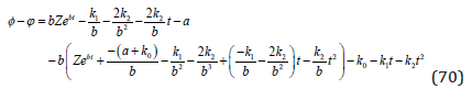
In other words, the CO₂ level in the atmosphere should really follow equation (65).

The general solution to the differential function has been determined. Furthermore, we have already determined the empirically relevant values of two parameters, a and b, from the empirical data. Now, we will study the future of the CO₂ level in the atmosphere, x(t), as a function of alternative levels of emissions and forestry activities. We define time zero as “the middle of year 2022”, namely July 1, 2022. Then, t=0. At that time, x(0) = x0. For alternative assumptions concerning emissions and forestry activities, we can also determine the parameters of the exogenous forcing function, f(.), namely k0, k₁ and k₂. With all of this information available, we can determine the final free parameter of the differential function, namely Z.
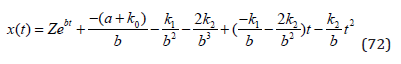
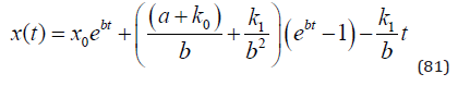
From (65), we get the general function of x(t):

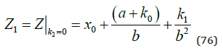
We introduce the initial condition, the value of x(t) at t=0.

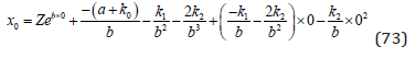
Now, we can determine Z as a function of the parameters:

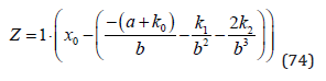
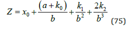
In the special case when k₂=0, we have:

Now, with this information about Z as a function of the parameters, we have:

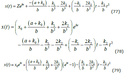
and the special case:

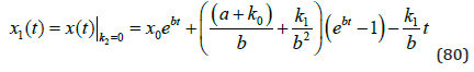
In (Figure 4), equation (80) is used to predict the CO₂ time path from 1990 to 2021. It is compared to the real observations. (Tables 1 & 2) contain the other parameters. The differential equation prediction follows the true development rather well, but underestimates the latest CO₂ levels slightly. One reason may be variations in the industrial emission increments. Still, the prediction model results replicate the true history rather well and we may believe in equation (80). In (Figures 5 & 6), we see the predictions of the future CO₂ development, from year 2022 until year 2100, based on equation (80) and alternative emission strategies. It is clearly possible to reduce or increase the future CO₂ concentrations very much, depending on the selected emission strategy. Note that, even if we select to reduce the emissions by 1.5 Gt/year, the CO₂ concentration in the atmosphere will continue to increase from the 2022 level during several years, before it starts to decrease.

Figure 4.The time path of the CO₂ level in the atmosphere, x, from year 1990 until 2021, in the empirical data, x_ppm_real, and the prediction, x_ppm_Lpred, via the solution to the differential equation (80), based on the assumptions that the initial CO₂ level in year 1990 and all other parameters are known. In year 1990, t = 0. Parameter k0 is the emission level in 1990, namely 22.729 (Gt) and k₁ = (the emissions in 2021 – the emissions in 1990) / (31 years). This calculation gives a k₁ value of approximately 0.4269 (Gt per year).

Figure 5.Emission strategy conditional predictions of the CO₂ level in the atmosphere, x (Gt), from year 2022 until 2100, via equation (80), based on the assumptions that the initial CO₂ level in year 2022 and all other parameters are known. In year 2022, t = 0, and the initial value x0 is estimated from the values in 2020 and 2021. (3250.11-3232.86) + 3250.11 = 3267.36 (Gt). Parameter k0 is the estimated emission level in 2022, assumed to be identical to the level in 2019, directly before the Corona pandemic, namely 37.911 (Gt). The time derivative of the emissions, k₁, takes alternative values, from -1.5 to + 1.0 (Gt per year). Tables 1 and 2 contain

Figure 6.Emission strategy conditional predictions of the CO₂ concentration in the atmosphere, x (ppm), from year 2022 until 2100, via equation (80), based on the assumptions that the initial CO₂ level in year 2022 and the parameters were known. In year 2022, t = 0, and the initial value x0 is estimated from the values in 2020 and 2021. (3250.11-3232.86) + 3250.11 = 3267.36 (Gt). Parameter k0 is the estimated emission level in 2022, assumed to be identical to the level in 2019, directly before the Corona pandemic, namely 37.911 (Gt). The time derivative of the emissions, k₁, takes alternative values, from -1.5 to + 1.0 (Gt per year). Tables 1 and 2 contain the other parameters.

The Decision k₁ and Effects on the Climate

As found in the already reported results, it is obvious that the future CO₂ level, and as a consequence the climate, will be affected by changes in the net emissions. Now, we will investigate how the parameter k₁ can be used as a tool in the climate control process and what the optimal decisions can be. We may consider the k₁ parameter as a decision variable, to be controlled by international political processes and to a considerable extent be a function of changes in industrial emissions of CO₂. The decision variable k₁ can also be influenced by increased activities in forestry, where earlier not managed forests in equilibrium, are transformed to sustainably managed forests. The increased harvest volumes can replace fossil fuels in Combined Heat and Power, CHP, plants, perhaps also combined with Carbon Capture and Storage, CCS, technology. The increased harvest volumes can also be used to produce construction materials that can store carbon for a long time. We may let this transformation process concern some constant number of hectares, each year, during a long sequence of years. When that happens, the net absorption of CO₂ sustainably increases and we may describe this as a reduction of k₁. In the same way, we may assume that we transform forestry in some other way, with genetically improved plants that grow faster, with more rational forest management decisions or with gradually increased used of fertilizers and/or irrigation.

Via all of these forestry changes, that we can denote sustainable forestry investments, we can each year, obtain a higher level of net growth, and net CO₂ absorption. This corresponds to a reduction of k₁. In order to simplify the exposition, from now on, we only consider cases where k₂ = 0. A corresponding but more page consuming treatment with arbitrary k₂ values may be developed by the interested reader.) Hence, we have:

The derivative of x with respect to k₁ is found in (82).

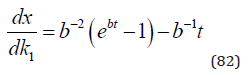
It is important to know if this derivative can be signed. The following procedure makes this possible:

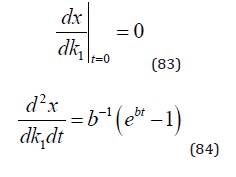
Now, we know that the derivative is zero for t=0 and increases with t. As a result, we get (86).

Hence, we know that the derivative of the CO₂ level with respect to k₁ is strictly positive, at every future point in time. As we see in equation (87), the derivative of the CO₂ level with respect to k₁ is a strictly increasing function of time.

If we are interested to control the climate via the CO₂ level, we should have some objective function that makes it possible to know how the utility is affected by the CO₂ level at different points in time. Let us consider a CO₂ path dependent utility function, which is scaled in such a way that it can be expressed in economic terms. In the rest of this paper, the expression “utility” should be understood as the total economic value of the utility, from t = 0 until t = T. Note that we are interested in the climate from t = 0 until some future point time, T.

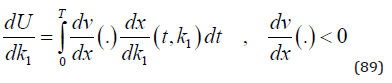
The marginal utility of increasing k₁ is found in (89). We assume that we prefer to have a colder climate, and for that reason want to have a lower CO₂ level in the atmosphere. In other words; The derivative of v with respect to x should be strictly negative.

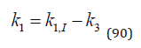
We assume that k₁ is a function of k₁,I and k₃, where the first part, k₁,I, is caused by changes in industrial emissions and the second part, k₃, is caused by increased net absorption of CO₂ in forests, because of investments in more productive and sustainable forestry.

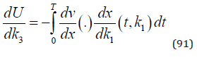
Obviously, the marginal utility of forestry investments (91), has the opposite sign compared to (89).

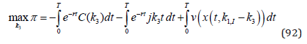
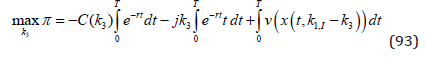
The forestry investment optimization problem is found in (92). C(k₃) is the investment cost function at a particular point in time during the investment process. The interest rate in continuous time is r. It is assumed that a particular level of “continuous investment” is selected, which for instance can mean that some new active forestry is started, each year, from time 0 until time T. Each year within this time interval, the area of “new forestry” increases with the same number of hectares. This type of action can for instance be made in very large regions in Canada and Russian Federation, where presently no active forestry can be found. It is natural to distribute such investments over time, in this way, since it takes considerable time to construct new infrastructure and to expand the capacities of industrial facilities and the labor force. The variable cost at time t is jk3t, where j is a new cost parameter.

Clearly, parts of the cost functions can be placed outside the integrals.

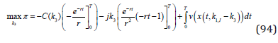
As we see in (94), the first two integral can be explicitly calculated.

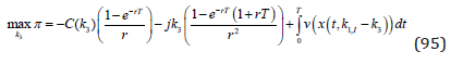
In (95), we have the optimization problem in explicit form.

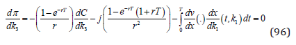
The first order optimum condition is:

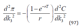
The second order derivative of the objective function with respect to the forestry investment level is shown in (97).

We assume that the rate of interest is strictly positive, that the investment process continues during a strictly positive time interval and that the cost function is strictly convex. In (98), we see that the objective function is a strictly concave function of the forestry investment level.

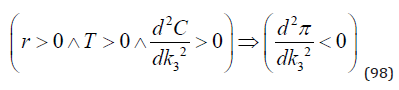
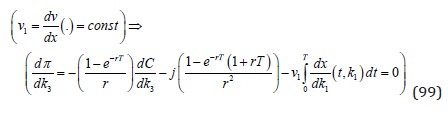
Hence, we have a unique maximum. Let us determine an explicit expression for the unique maximum. We assume that the derivative of the utility function with respect to the CO₂ level is constant, namely v1. Alternative assumptions can of course be made, if some empirical facts can be shown to support such assumptions. The resulting first order optimum condition is found in (99).

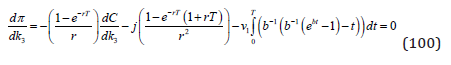
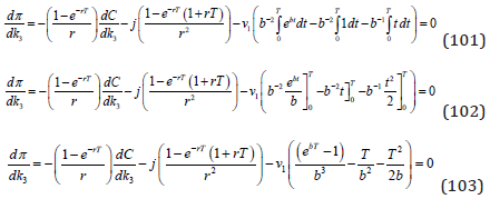
Now, since we already know the derivative of the CO₂ level with respect to k₁, from (82), we get (100).

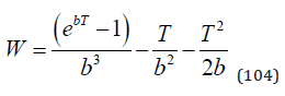
(100) can be further developed to (101), (102) and (103).

The last part of the expression (103) deserves a special treatment. We define that as W in equation (104). We are interested to determine the sign of W.

In (105), we find that W = 0 for T = 0. Equations (106), (107) and (108) make sure that W is strictly positive for strictly positive T.

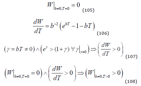
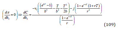
From equation (103), we get the optimal value of the marginal cost of the investment level, in (109). Since this marginal cost is a monotonically increasing function of the investment level, it will soon be possible to determine the optimal investment level from this value.

We assume that the optimal value of the marginal investment cost function is strictly positive (110).

We assume that the investment cost function can be approximated as a quadratic function. When empirical data becomes available, the parameters can be estimated.

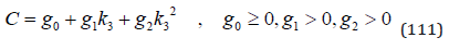
We also assume that the fix cost, g0, is comparatively small and does not make it more profitable to avoid all investments studied in this article. This is of course an empirical question, but in typical cases, g0 should be small. The marginal cost is found in (112).

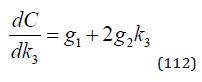
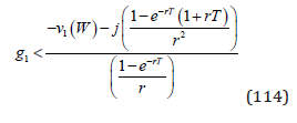
(109) and (112) lead to (113).

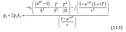
We assume that the parameter g1 is sufficiently small to motivate a strictly positive investment level. (It is easy to show that, in an earlier “forestry investment equilibrium”, obtained when the utility of climate change was not considered, the investments took place until the marginal cost of expansion was equal to the marginal revenue of increased access to forest areas. Hence, this argument tells us that g1 can be expected to be very close to zero. This makes it highly probable that (114) is relevant.

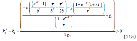
Then, the unique and strictly positive optimal investment in higher CO₂ absorption via forestry is given in (115).

A model is just an approximation of some part of reality. Hence, we can never expect to cover every detail of real problems. Nevertheless, it was possible to theoretically model and describe the natural CO₂ system as a rather simple first order differential equation, where the absorption is proportional to the CO₂ concentration. The logic behind such a model is easy to understand, based on fundamental physics, and the solution can be obtained with standard methods. It was also possible to estimate the parameters with high precision, based on publicly available empirical data. The t-values were rather high and the p-values were well below the 95% significance levels. Furthermore, it was possible to use the estimated differential function to derive a function describing the time path of the CO₂ concentration. This time path turned out to give a good picture of the real empirical time series. With the estimated differential equation, it was also possible to determine the existence of a unique and stable equilibrium. With the estimated parameter values, this equilibrium was calculated to be close to 262 ppm. In an earlier study, with a shorter time series, and with a simpler estimation method, Lohmander [12] derived an equilibrium of 280 ppm. Exactly the equilibrium 280 ppm was also reported by Solomon, et al. [11] to be the estimated pre-industrial equilibrium. We should be aware that the estimated equilibrium values 262 ppm and 280 ppm are close to each other. The estimated parameter values in the differential equation contain error terms with reported standard deviations.

Hence, 262 ppm, 280 ppm or some other equilibrium in the neighborhood of these values, should be expected to be the “pre-industrial equilibrium”. The exact equilibrium can probably never be determined without error.

It was possible to determine the future time path of the CO₂ concentration as a function of future industrial emission strategies, until year 2100. Of course, we will not know if these predictions were correct before we reach year 2100. On the other hand, such predictions may be used as tools in international emission reduction negotiations. Then, a key is that it is possible to make the negotiating partners understand and believe in the methodology (Appendix Figures 1-4). It is the firm opinion of the author of this paper that it should be possible to convince well educated negotiation delegations from different countries about the fundamental structure of these predictions and the mathematics behind it. Finally, the optimal investment intensity rule, equation (115), is a tool that hopefully does not only give a particular value, but also makes the users aware of the fundamental importance of some facts. It explicitly shows that some pieces of information are necessary to know, if we want to take optimal decisions. We have to know the parameters of the investment cost and the variable cost functions, the rate of interest in the capital market, the absorption parameter b in the CO₂ differential equation and the length of the time interval of interest. However, we also really need to know v1, the economically specified “marginal utility” of the CO₂ concentration.

Appendix Figure 1.

Appendix Figure 2.

Appendix Figure 3.

Appendix Figure 4.

In other words, as a first step, we have to know, and agree about, the economic value of decreasing the CO₂ concentration by 1 ppm. If we can not agree about that, we will not agree about rational investment levels in emission reductions and/or optimal areas of intensified forestry (Appendix Tables 1-3). For these reasons, the author hopes and suggests that United Nations initiates an international research and negotiation process where the fundamental principles and facts of relevance to managing the CO₂ concentration problem are in focus. In this work, the analyses and results presented in this paper can hopefully be useful as a starting point.

Appendix Table 1a: Data related to the analysis.

Appendix Table 1b: Data Definitions

Appendix Table 2: Regression in Gt.

Appendix Table 3: Regression in ppm.

It is possible to model the dynamics of the CO₂ level in the atmosphere via a differential equation. The formulated hypotheses, of how the CO₂ level is affected by natural emissions and concentration dependent absorption, could not be rejected. The parameters were empirically estimated, with high precision, from the latest available empirical time series of observations of CO₂ concentration in the atmosphere, and industrial emissions. It is possible to determine the time path of the CO₂ concentration of the natural system without industrial emissions, for arbitrary initial conditions. This system has a unique and stable equilibrium, with an expected estimated value of 262 ppm. With constant industrial emissions, the equilibrium would be found at a higher level, according to an explicit equation. Comparative statics analysis shows how the equilibrium is affected by alternative parameter adjustments. An extended version of the natural differential equation, with a forcing function, a quadratic function of time, representing the time paths of industrial emissions, has been developed. The general function of the time path of the CO₂ concentration of the natural system under the influence of industrial emissions, has been determined for arbitrary initial conditions and parameters of the industrial emission function. The CO₂ time path function has been analytically verified and empirically tested and found to be able to reproduce the historical CO₂ observations with high precision.

The time paths of the future CO₂ concentrations have also been calculated, for six alternative levels of change of the industrial emissions, from -1.5 Gt/year to +1.0 Gt/year, from the year 2022 until 2100. The net CO₂ emissions can be reduced over time, if sustainable forestry is gradually intensified. The rational intensity of this investment process has been determined. An explicit function for the optimal forestry intensification level, based on all CO₂ time path function parameters, the marginal cost of the CO₂ concentration, time interval parameters, rate of interest and cost function parameters, has been derived.

1. (2022) NOAA. Global Monitoring Laboratory, Earth System Research Laboratories, Trends in Atmospheric Carbon Dioxide, Mauna Loa CO₂
2. EDGAR, Crippa M, Guizzardi D, Solazzo E, Muntean M, et al. (2021) GHD emissions of all world countries - 2021 Report, EUR 30831 EN, Publications Office of the European Union, Luxembourg.
3. Brown S, Sathaye J, Cannell M, Kauppi PE (1996) Mitigation of carbon emissions to the atmosphere by forest management. The Commonwealth Forestry Review 75(1): 80-91.
4. Favero A, Daigneault A, Sohngen B (2020) Forests: Carbon sequestration, biomass energy, or both? Science Advances 6(13): eaay6792.
5. Forster EJ, Healey JR, Dymond C, David S (2021) Commercial afforestation can deliver effective climate change mitigation under multiple decarbonisation pathways. Nature Communications 12: 3831.
6. Holmgren P (2021) The forest carbon debt illusion, Future Vistas AB.
7. Lohmander P (2020b) Optimization of continuous cover forestry expansion under the influence of global warming, International Robotics & Automation Journal, Volume 6(3): 127-132.
8. Lohmander P (2020c) Fundamental principles of optimal utilization of forests with consideration of global warming, Central Asian. Journal of Environmental Science and Technology Innovation 1(3): 134-142.
9. Lohmander P (2020a) Dynamics and control of the CO₂ level via a differential equation and alternative global emission strategies. Int Rob Auto J 6(1): 7-15.
10. Braun M (1986) Differential Equations and Their Applications. Applied Mathematics Sciences, Springer 15: 546.
11. Solomon S, Qin D, Manning M, Zena C, Melinda M, et al. (2007) Climate Change 2007-The Physical Science Basis. Contribution of Working Group I to the Fourth Assessment Report of the Intergovernmental Panel on Climate Change. bridge University Press.
12. Hatami N, Lohmander P, Moayeri MH, Soleiman ML (2020) A basal area increment model for individual trees in mixed continuous cover forests in Iranian Caspian forests. J For Res 31: 99-106.
13. Fagerberg N, Lohmander P, Eriksson O, Olsson JO, Poudel BC, et al. (2022) Evaluation of individual-tree growth models for Picea abies based on a case study of an uneven-sized stand in southern Sweden. Scandinavian Journal of Forest Research 37(1): 45-58.
14. Lohmander P (2020d) Adaptive mobile firefighting resources: Stochastic dynamic optimization of international cooperation. Int Rob Auto J 6(4): 150-155.
15. Lohmander P (2020e) Forest fire expansion under global warming conditions: -Multivariate estimation, function properties and predictions for 29 countries. Cent. Asian J Environ Sci Technol Innov 1(5): 262-276.
16. Mohammadi Z, Lohmander P, Kašpar J, Roman B, Jaroslav H, et al. (2021) The effect of climate factors on the size of forest wildfires (case study: Prague-East district, Czech Republic). J For Res.
17. Lohmander P (2021a) Optimization of Forestry, Infrastructure and Fire Management. Caspian Journal of Environmental Sciences 19: 287-316.
18. Lohmander P (2021b) Optimization of distance between fire stations: effects of fire ignition probabilities, fire engine speed and road limitations, property values and weather conditions. Int Rob Auto J 7(4): 112-120.
19. Lohmander P (2021c) Global Stability via the Forced Global Warming Equation, Fire Control with Joint Fire Fighting Resources, and Optimal Forestry, KEYNOTE at ICASE 2021: International Conference on Applied Science & Engineering.
20. O Hara F Jr (1990) Carbon Dioxide and Climate, (3^rd)., Tennessee, Oak Ridge.