The Log-Generalized Gamma Burr III Regression Model with Application to Predict Death of Breast Cancer Volume 46- Issue 5

Olobatuyi Kehinde Ibukun¹*, Asiribo Osebekwiin Ebenezer² and Talabi Olusola Adetunji³

• ¹University of Milano-Bicocca, Milan, Italy Department of Statistics, Italy
• ²Federal University of Agriculture, Abeokuta Department of Statistics, Nigeria
• ³Federal University of Agriculture, Abeokuta Health Centers, Nigeria

Received: October 19, 2022;   Published: October 31, 2022

*Corresponding author: Olobatuyi Kehinde Ibukun, University of Milano-Bicocca, Milan, Italy Department of Statistics, Italy

DOI: 10.26717/BJSTR.2022.46.007423

Abstract PDF

We study the properties of the called log-generalized gamma Burr III distribution defined by the logarithm of the generalized gamma Burr III random variable (Olobatuyi, et al. [1]). An advantage of the new distribution is that it includes as special sub-models classical distributions reported and has the ability to model unimodal HFs. We obtain formal expressions for the moments, moment generating function, quantile function and mean and median deviations. We constructed a regression model based on the new distribution to predict relief time of headache patients and death of breast cancer patients treated by mastectomy. It can be applied to censored data since it represents a parametric family of models that includes as special sub-models several widely known regression models. The regression model was fitted to a data set of 1207 eligible breast cancer patients. We predict survival probability after the mastectomy in terms of highly significant clinical and pathological explanatory variables associated with the death of the patients. The predicted probabilities of survival are calculated under two nested models.

Keywords: Generalized Gamma Burr III Distribution; Censored Data; Log- Generalized Gamma Burr III Distribution; Log- Generalized Gamma Burr III Regression Model; Survival Function

Standard lifetime distributions usually present very strong restrictions to produce bathtub curves, and thus appear to be inappropriate for interpreting data with this characteristic. Some distributions were introduced to model this kind of data, as the exponential power family [2], the beta integrated model [3], and the generalized log-gamma distribution, among others. A good review of these models is described, for instance, in [4] In the last decade, new classes of distributions for modeling this type of data based on extensions of the Weibull distribution were developed. For example, the exponentiated Weibull (EW) (Mudholkar, et al. [5]), the additive Weibull [6], the modified Weibull (Lai, et al. [7]), the beta Weibull (BW) (Famoye, et al. [8,9]) and the generalized modified Weibull (Carrasco, et al. [10]) distributions. Further, (Carrasco, et al. [10]) investigated several mathematical properties of the BW geometric distribution, which is a highly flexible lifetime model to cope with different degrees of kurtosis and asymmetry. The Generalized Gamma Burr III (GGBIII) distribution, due to its flexibility in accommodating the different types of the risk function depending on its parameters, can be used in a variety of problems in modeling survival data. The main motivation for the use of the GGBIII model is that it contains as special sub-models several distributions such as the generalized gamma Fisk, Zografos and Balakrishnan-Burr III, Zografos and Balakrishnan-Fisk, Burr III distribution among others. Also, it was reported that gamma model is the most effective model for analyzing highly skewed data such as survival data, [11].

Breast cancer presents a major risk to American women, who have a 1 in 8 lifetime chance of developing the disease. The estimated incidence of invasive breast cancer in the United States for 2010 was 207,090 women, making it the most common cancer after skin cancer in women. Although survival has improved because of advances in treatment and early diagnoses as a result of the increased use of mammographic screening, fatalities in 2010 have been put at 40,000. Mastectomy is surgery that removes the entire breast. All the breast tissue is removed, sometimes along with other nearby tissues. If just the breast is removed (and not lymph nodes under the arm) it is called a simple (or total) mastectomy. A simple mastectomy combined with an axillary lymph node dissection (discussed below) is called a modified radical mastectomy. The primary end point was survival (DFS), defined as time to the earliest of either death (all-cause), or last follow-up. The follow-up period was defined as time to the earliest of either death (all-cause), or last follow-up. For the first time, we propose a log-generalized gamma Burr III regression model to predict the 𝑡 months survival probability after mastectomy in terms of highly significant clinical and pathological variables associated with death of the patient after surgery. The study cohort comprises 1207 patients with clinically localized cancer treated by mastectomy. The data consist of the random response variable given by the number of months (𝑦𝑖) after mastectomy. Uncensored observations correspond to patients having death time computed. Censored observations correspond to patients who were not observed to have died at the time the data were collected. The numbers of censored and uncensored observations are 1135 and 72, respectively, of the total of 1207 patients.

In this article, we propose a location-scale regression model based on the LGGBIII distribution, referred to as the LGGBIII regression model, which is a feasible alternative for modeling the existing types of failure rate functions. Some inferential issues were carried out using the asymptotic distribution of the maximum likelihood estimators (MLEs). The sections are organized as follows. In Section 2, we define the LGGBIII distribution. Mathematical properties of this distribution are investigated in Section 3. In Section 4, we obtain the order statistics. We propose a LGGBIII regression model for censored data and discuss inferential issues in Section 5. In Section 6, a breast cancer data set is analyzed to show the flexibility, practical relevance and applicability of our regression model. Section 7 ends with some concluding remarks.

Generalized Gamma Burr III Distribution

Most generalized Burr III distributions such as Beta Burr III distribution Antonio and Silva (2014) have been proposed in reliability literature to provide better fitting of certain data sets than the traditional two and three parameter Burr III models. The GGBIII density function (Olobatuyi, et al. [1]) with five parameters 𝛼 > 0, 𝛽 > 0, 𝛿 > 0, 𝑘 > 0 and 𝜆 > 0 is given by (𝑡 > 0)

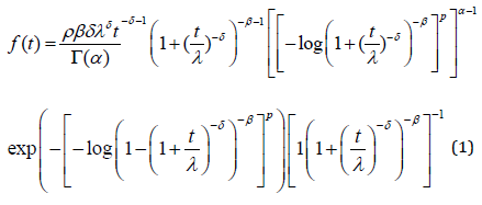
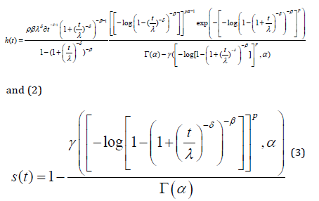
where Γ(. ) is a gamma function. Here, α and k are two additional shape parameters to the Burr III distribution to model the skewness and kurtosis of the data. The important characteristic of the GGBIII distribution is that it contains as special sub-models. The hazard and survival rate functions corresponding to (1) are

Shape of GGBIII Distribution

Plots of the density function of the Generalized Gamma Burr III distribution for selected parameters values are given in Figure 1. The plot indicates that the GGBIII distribution can be decreasing or right skewed.

Figure 1

The Log-Generalized Gamma Burr III Distribution

In this section, log-generalized gamma Burr III distribution is introduced. It is based on the logarithm of the continuous GGBIII distribution that is presented above. The log-generalized gamma Burr III distribution is proposed and denoted as LGGBIII. Some of its mathematical properties are studied, estimation by the method of maximum likelihood is discussed, and applications to two real datasets are described. The new distribution is shown to outperform at least two models which are the log-ZBD and Cox model. Let 𝑇 be a random variable having the GGBIII density function (1), The random variable 𝑌 = log(𝑇) has a log-generalized gamma-Burr II(LGGBIII) distribution, whose density function is reparametrized in

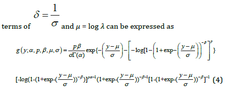
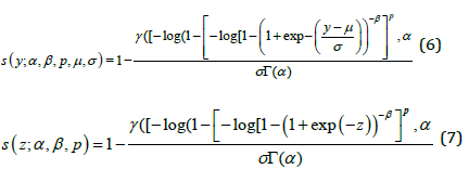
Where − ∞ < 𝑦 < ∞, 𝜎 > 0, and −∞ < 𝜇 < ∞ , 𝑝 > 0, 𝛼 > 0, 𝛽 > 0. We refer to the new model (4) as the LGGBIII distribution, say 𝐿𝐺𝐺𝐵𝐼𝐼𝐼(𝛼, 𝛽, 𝑝, 𝜇, 𝜎 ) where 𝜇 is a location parameter, 𝜎 is a dispersion parameter and 𝛼, 𝛽 and 𝑘 are shape parameters. The following results hold if 𝑇 ∼ 𝐺𝐺𝐵𝐼𝐼𝐼(𝛼, 𝛽, 𝑝, 𝛿, 𝜆) then 𝑌 = 𝑙𝑜𝑔(𝑇) ∼ 𝐿𝐺𝐺𝐵𝐼𝐼𝐼(𝛼, 𝛽, 𝑝, 𝜇, 𝜎 ). The standard random variable 𝑍 = 𝑌 − 𝜇 ⁄𝜎 with density function is defined as

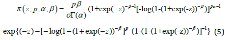
The special case of the model lead to a standard log-ZBD (LZBD new) distribution for 𝑝 = 1. For 𝛽 = 𝑝 = 1, we obtain the log-Zografos and Balakrishnana Fisk (LZB-F new). The survival functions corresponding to (4) and (5) are

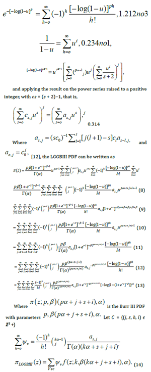
Expansions of Density Functions

If a random variable 𝑍 has the LGGBIII density, we say 𝑍~𝐿𝐺𝐺𝐵𝐼𝐼𝐼(𝛼, 𝛽, 𝑘 ). Let 𝑢 = (1 + 𝑒−𝑧)−𝛽, and then using the series representation from Gradshteyn and Ryzhik (2000).

Shape of LGGBIII Distribution Function

The plot (4) in Figure 1 for selected parameter values show great flexibility of the density function in terms of the parameters α, β, 𝑝 in Figure 2a β = 3, 𝑝 = 2 and in Figure 1b, α = 2.5, 𝑝 = 2 and in Figure 1d, α = 2.5, β = 3.

Figure 2

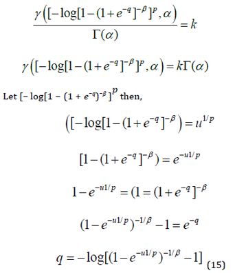
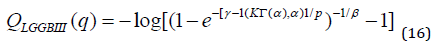
LGGBIII Quantile Function

We now give an expansion for the quantile function 𝑞 = 𝐹−1(𝑘) (given k) of the LGGBIII distribution. First, we have k = F(q). It is possible to obtain as function of p from some expansions for the inverse of the gamma incomplete function 𝑄_{𝐺𝐺𝐵𝐼𝐼𝐼}(𝑞) = 𝑘, 0 < 𝑞 < 1.

Moments, Moment Generating Function Mean and Median Deviations

In this section, we present the moments, moment generating function, mean and median deviations for the GGBIII distribution.

Moments and Moment Generating Function

As with any other distribution, many of the interesting characteristics and features of the LGGBIII distribution can be studied through the moments. Let 𝛽∗ = 𝛽(𝑝𝛼 + 𝑗 + 𝑠 + 𝑖), and 𝑋~ 𝐿𝐵𝐼𝐼𝐼(𝜇, 𝜎, 𝛽∗). Then the 𝑟𝑡ℎ moment of the random variable 𝑌 is

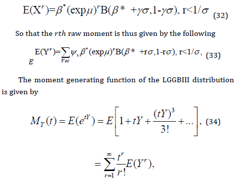
Mean and Median Deviations

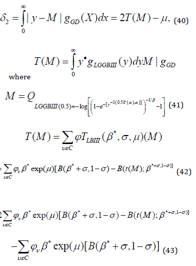
Mean Deviation: If Y has the LGGBIII distribution, we derive the mean deviation about the mean 𝜇 by

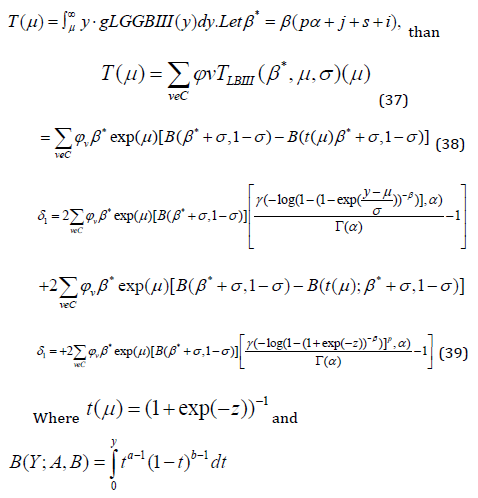
Median Deviation: If 𝑌 has the LGGBIII distribution, we derive the median deviation about the median 𝑀 by

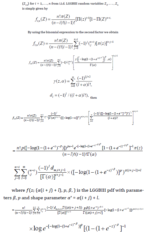
Order Statistics of LGGBIII Distribution

Order statistics make their appearance in many areas of statistical theory and practice. The density f _i:n( x) of the i^th order statistic

The Log-Generalized Gamma Burr III Regression Model

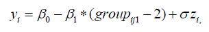
In many practical applications, the lifetimes are affected by explanatory variables such as the cholesterol level, blood pressure, weight and many others. Parametric regression models to estimate univariate survival functions for censored data regression problems are widely used. A parametric model that provides a good fit to lifetime data tends to yield more precise estimates of the quantities of interest. Based on the LGGBIII density function, we propose a linear location-scale regression model linking the response variable 𝑦_𝑖 and the explanatory variable vector 𝑉_𝑇 = (𝑣_𝑖1, … , 𝑣_𝑖𝑝) as follows

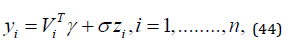
where the random error 𝑧𝑖 has density function (40), 𝜸 = (𝐵₁, … , 𝐵_𝑝), 𝜎 > 0, 𝑝 > 0, 𝛼 > 0, 𝛽 > 0 are unknown parameters. 𝜇𝑖 = 𝑉^𝑇𝜸 is the location of 𝑦_𝑖 . The location parameter vector 𝝁 = (𝜇₁, … . , 𝜇_𝑛) 𝑇 is represented by a linear model 𝝁 = 𝑽_𝜸, where 𝑽 = (𝒗_𝟏, … , 𝒗_𝑛) 𝑇 is a known model matrix. Let 𝐹 and 𝐶 be the sets of individuals for which 𝑦𝑖 is the log-lifetime and log-censoring, respectively. The log-likelihood function for the vector 𝜽 = (𝛼, 𝛽, 𝑝 , 𝜎, 𝛾_𝑇)𝑇of parameters from model (39) has the form

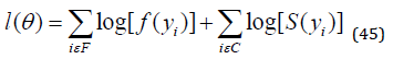
where 𝑓(𝑦_𝑖) is the density function (4) and 𝑆(𝑦_𝑖) is the survival function (5) of 𝑌_𝑖. The log-likelihood function for 𝜽 reduces to

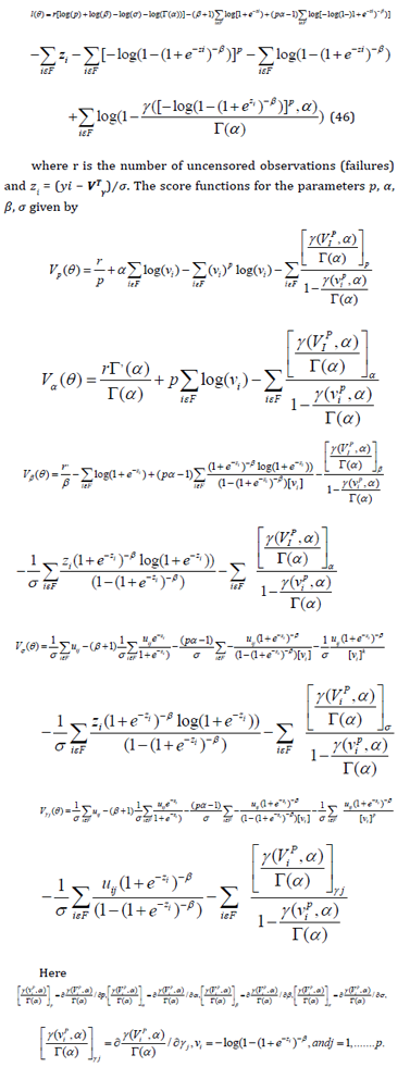
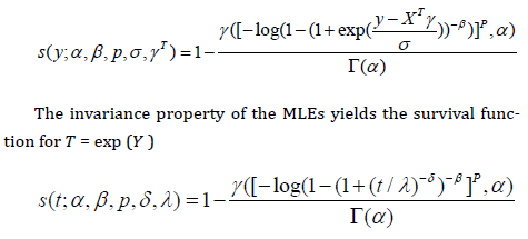
The MLE 𝜽̂ of the vector 𝜽 of unknown parameters can be calculated by maximizing the log-likelihood (46). We use the subroutine NLMixed in SAS to calculate 𝜽̂. Initial values for and can be taken from the fit of the log-Zog Fisk (LZFisk) regression model with 𝛽 = 𝑝 = 1. The fitted LGGBIII model gives the estimated survival function of Y for any individual with explanatory vector x

The approximate multivariate normal distribution 𝑁𝑝+5(0, 𝐋(𝜽)−1) for 𝜽 ̂ can be used in the classical way to construct approximate confidence regions for some parameters in 𝜽. We can use the likelihood ratio LR statistic for comparing some special sub-models with the LGGBIII model. We consider the partition 𝜽 = (𝜽_𝑻, 𝜽_𝑻) 𝑻where 𝜽 is a subset of parameters of interest and 𝜽 2 is a subset of remaining parameters. The LR statistic for testing the null hypothesis 𝑯_𝟎:𝜽₁=𝜽₁⁽⁰⁾ versus the alternative hypothesis 𝑯_𝟎:𝜽₁≠𝜽₁ ⁽⁰⁾ is given by 𝜔=2{ℓ(𝜽̂)−ℓ(𝜽̃)} where where 𝜽 ̃ and 𝜽̂ are the estimates under the null and alternative hypotheses, respectively. The statistic 𝜔 is asymptotically (as 𝑛→∞) distributed as 𝜒_ℎ ² where ℎ is the dimension of the subset of parameters of interest.

Predicting the Time to Headache Relief

Thirty-eight patients are divided into two groups of equal size, and different pain relievers are assigned to each group. The outcome reported is the time in minutes until headache relief. The variable censor indicates whether relief was observed during the observation period (censor = 0) or whether the observation is censored (censor=1).

The variables involved in the study are
• 𝑡𝑖 − survival time to Headache relief (in minutes);
• 𝑐𝑒𝑛𝑠𝑖 − censoring indicator (0 𝑜𝑟 1);
• 𝑔𝑟𝑜𝑢𝑝𝑗 − (𝑗 = 1,2);
Now, by fitting the model

𝐻0: 𝑔𝑟𝑝 1 𝑡 𝑖𝑚𝑒 = 𝑔𝑟𝑝 2𝑡𝑖𝑚𝑒 𝑣𝑠 𝐻1: 𝑔𝑟𝑝 1 𝑡 𝑖𝑚𝑒 < 𝑔𝑟𝑝 2 𝑡 𝑖𝑚𝑒 The random variable 𝑧𝑖 follows the LGGBIII distribution (5) for 𝑖 = 1, … ,38. We are interested in modelling which group recovers faster. The MLEs of the model parameters are calculated using the procedure NLMIXED in SAS. Iterative maximization of the logarithm of the likelihood function (46) starts with initial values for 𝛽0 = 𝛽1 = 1, 𝛼 = 1, 𝛽 = 1, 𝑝 = 1, 𝜎 = 1, to fit the regression model. Table 1 lists the Maximum Likelihood Estimation of the model parameters. The value of Akaike Information Criterion (AIC), Corrected Akaike Information Criterion (AICc), and Bayesian Information Criterion (BIC) statistics are smaller for LGGBIII regression model. A comparison of the new model with one of its sub-models which is LZB-D model and most useful model for fitting survival data which is Log-Weibull (LW) model using LR statistic is presented in Table 2 together with p-values. From the values of these statistics, LGGBIII distribution provided a good fit for this data. The LGGBIII regression model outperforms the other models irrespective of the criteria and it can be used effectively in the analysis of these data. So, the proposed model is a great alternative to model survival data. The model to know which group has a high rate of Headache relief that is the group that has a short time to Headache relief was fitted, recall that log(𝜆) = 𝜇 then, since 𝜇 = 𝑣^𝑇𝖰 say log(𝜆) = 𝑏₀ − 𝑏₁ × (𝑔𝑟𝑜𝑢𝑝 − 2) as the mean of the 𝑦_𝑖 . Now, from the result provided in Table 3 then substituting the value of 𝑏0 and 𝑏1 into the regression model as follows. For group 1

Table 1: MLEs of the Model Parameters for the Time –To- Headache Relief.

Table 2: The -2L, AIC, AICC, BIC of Time of Headache Relief.

Table 3: The Likelihood Ratio Test Statistic.

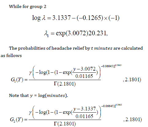
These probabilities calculated at the observed times are shown for the two groups in Table 4.
Since the slope estimate is negative i.e. 𝑏1 = −0.1265 , 𝑆𝐸 = 0.02272 then 𝑡 value = −5.57 with p-value of < 0.0001, it was seen that group 1 has a shorter time to Headache relief than group 2 that is pain reliever 1 leads to overall significantly faster relief, but the estimated probabilities give no information about patient-to-patient variation within and between groups. For example, while pain reliever 1 provides faster relief overall, some patients in group 2 may respond more quickly than other patients in group 1. Provided below in Figures 3 & 4 is a graphical representation of the predicted value for the two groups.

Table 4: The predicted value of the Time to Headache Relief.

Figure 3

Figure 4

Predicting Time-to-Death of Breast Cancer Patient

The study cohort comprises 1207 patients with cancer treated by mastectomy. The data consist of the random response variable given by the number of months (𝑦𝑖) after mastectomy. Uncensored observations correspond to patients having death time computed. Censored observations correspond to patients who were not observed to have died at the time the data were collected. The numbers of censored and uncensored observations are 1135 and 72, respectively, of the total of 1207 patients. The following explanatory variables were associated with each patient (for 𝑖 = 1, … . , 1207):

• 𝛿_𝑖 ∶ is the event indicator where 1 represents the event (death) and 0 is censored;
• 𝑝𝑎𝑡ℎ𝑐𝑎𝑡: is the size of the pathologic tumor
• 𝑒𝑠𝑡: is the estrogen receptor status (0=negative, 1=positive, unknown= 2)
• 𝑝𝑟: is the progesterone receptor status (negative = 0, positive = 1, unknown = 2)
• 𝑝𝑎𝑡ℎ𝑜𝑙𝑜: is the tumor size category in centimeter (0, <=2, 2-5, >5)
• 𝑙𝑛𝑖: is the lymph node involvement (0 =no, 1= yes)
• ℎ𝑔: is the histologic grade (grade 1, grade 2, grade 3, unknown = 4)
• 𝑖𝑛𝑝𝑜𝑠: is the positive axillary lymph node. Now, we present the result by fitting the model

where the dependent variable 𝑦𝑖 follows the LGGBIII density function (4) for 𝑖 = 1, … , 1207. The MLEs of the model parameters was calculated using routine NLMIXED in SAS package. Iterative maximization of the logarithm of the likelihood function starts with initial values for and taken from the fit of the L regression model with 𝑝 = 1. Tables 5 & 6 lists the MLEs of the parameters for the LGGBIII and LZBD regression models fitted to the current data. The LR statistic for testing the hypothesis that 𝐻0 : p = 1 versus 𝐻1: 𝐻0 is not true, i.e., to compare the LGGBIII and LZBD regression models, is 𝑤 = 2{542.5 − 524.8} = 17.70 (p-value < 0.0001), which gave favorable indications toward to the LGGBIII model. A comparison of the new model with its sub-model using AIC, AICc, and BIC criteria was performed in Table 7. From the values of these statistics, LGGBIII distribution provides a good fit for these data. The fitted LGGBIII regression model indicates that not all explanatory variables are significant at 5%. [13] proposed a very useful regression model for analyzing censoring failure times, where the random variable of interest represents failure time and the failures times are assumed identically distributed in some specified form. He noted that if the proportional hazards assumption holds (or, is assumed to hold) then it is possible to estimate the selected parameter(s) without any consideration of the hazard function (non-parametric approach). This approach to survival data is called proportional hazards model. The Cox model may be specialized if a reason exists to assume that the baseline hazard follows a parametric form. In this case, the baseline hazard can be replaced by a parametric density. Typically, we can then maximize the full likelihood which greatly simplifies model fitting and provides interpretability at the cost of flexibility. From the result of the regression model, it was observed that not all the explanatory variables are significant that is size of the pathologic tumor, positive auxiliary lymph node, and the tumor size category in centimeter are significant at 5% and they are used to predict the survival time of the patients. Based on these three significant variables, MLEs for this new model were presented [14,15].

Table 5: MLEs of the parameters for the LGGBII and LZBD regression models fitted to the Breast Cancer data.

Table 6: MLEs of the parameters for the Cox regression models fitted to Breast Cancer data.

Table 7: AIC, BIC and AICC statistics for comparing the LGGBIII, LZBD and Cox models.

Table 8: Survival for randomly selected patients’ probability.

Table 9: The Significant value of Breast Cancer data LGGBIII Regression Model.

From Table 9, we have 𝛼 = 1.499, 𝛽 = 1.734, 𝑝 = 0.156, 𝛿 = 1/ 𝛿 = 4.425,

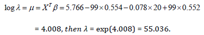
So, the survival probability of this patient say 𝑡 = 200 𝑚𝑜𝑛𝑡ℎ𝑠 by inserting the parameters in equation above we have

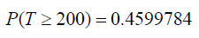
That is the patient 1113 has chance of 46% of surviving past these months. Evidently, the survival probability converges to zero when the linear predictor 𝜇_𝑖 = exp(𝑋𝑇𝖰) tends to −∞ and converges to one when the linear predictor goes to +∞. In other words, the death of patients with breast cancer treated by mastectomy for a fixing time 𝑡 after the surgery, approaches one (zero) when the linear predictor increases to a very large negative (positive) number. We consider ten hypothetical patients who underwent mastectomy having fixed values for the explanatory variables given below

A new class of generalized Burr III distribution called the generalized gamma-Burr III distribution was proposed and studied. The GGBIII distribution has the family of Zografos and Balakrishnan distribution as special cases. The density of this new class of distributions was expressed as a linear combination of Burr III density functions. The GGBIII distribution was established to possess hazard function with flexible behavior. We also obtained closed form expressions for the moments, mean and median deviations, and distribution of order statistics. Maximum likelihood estimation technique was used to estimate the model parameters. To further the previous work, in this work, we built on the log transformation of GGBIII distribution proposed in our previous work. The main motivation was to predict the survival probability of breast cancer patients after surgery called mastectomy. The name of the log transformation is Log-Generalized Gamma Burr III (LGGBIII) model. We compared the proposed log-transform model with existing models such as Log-Zografos-Balakrishnan model Log- Weibull model and Cox model. Before the prediction, it has been established in the previous work that GBBIII distribution fitted better than its competitors. This work only confirms our curiosity in predicting time – to – death of breast cancer patients. We randomly selected 10 patients and calculated their survival probability which was also visualized in the figure above. Additionally, we analyzed two groups of patients with headaches. Also, predicted the time – to – headache relief as shown in the table. In general, the proposed LGGBIII model has higher predictive power compared to its competitors as established by different goodness of fit tests.

The authors would like to express their sincere gratitude to all those who have contributed in one way or the other towards the success of this paper.

1. Olobatuyi K I, Asiribo O E, Dawodu G A (2018) A New Class of Generalized Burr III Distribution for Lifetime Data. International Journal of Statistical Distributions and Applications. Vol. 4(1): 6-21.
2. Smith R, Bain L (1975) An Exponential Power Life-Testing Distribution. Communications in Statistics-Theory and Methods 4: 469-481.
3. Hjorth U (1980) A reliability distribution with increasing, decreasing, constant and bathtub failure rates. Human and Ecological Risk Assessment Technometrics 22: 99-107.
4. Rajarshi S M B (1988) Bathtub distributions. Communications in Statistics, Theory and Methods 17: 2597-2521.
5. Mudholkar G S, Srivastava D K, Friemer M (1995) The exponentiated Weibull family: A reanalysis of the bus-motor- failure data. Technometrics 37(4): 436-445.
6. Xie M, Lai C D (1996) Reliability analysis using an additive Weibull model with bathtub shaped failure rate function. Reliability Engineering and System Safety 52(1): 87-93.
7. Lai C D, Xie M, Murthy D N (2003) A modified Weibull distribution. Transactions on Reliability, 52: 33-37 Lawless, J. F. 2003. Statistical Models and Methods for Lifetime data. Wiley, New York.
8. Famoye F, Lee C, Olumolade O (2005) The beta-Weibull distribution. Journal of Statistical Theory and Applications 4: 121-136.
9. Lee C, Famoye F, Olumolade O (2007) Beta-Weibull distribution: some properties and applications to censored data. Journal of Modern Applied Statistical Methods 6: 173-186.
10. Carrasco J M F, Ortega E M, Cordeiro G M (2008) A generalized modified Weibull distribution for lifetime modeling. Computational Statistics and Data Analysis 53(2): 450-462.
11. Marcelino P, Ortega EM, Cordeiro G M (2011) The Kumaraswamy generalized gamma distribution with application in survival analysis. Statistical methodology 8.5: 411-433.
12. Gradshteyn I S, Ryzhik I M (2000) Table of Integrals, Series, And Products (7^th ).,
13. Cox D R (1972) Regression models and life tables (with discussion). Journal of the Royal Statistical Society: Series B (Statistical Methodology) 34(2): 187-220.
14. Antonio E G, da-Silva C Q (2014) The Beta Burr III Model for Lifetime Data. 1 – 33. Brazil.
15. Cordeiro GM, Giovana O S, Ortega E M (2011) The Beta Extended Weibull Family, p. 1-29.