 Review Article
Abstract
In this paper we analyze a mathematical model of cancer cell invasion consisting of a system of partial differential equations which describes the interactions between cancer cells, the matrix degrading enzyme and the host tissue. The main objective of the present paper is to show, using numerical computations, the ability of a relatively simple model to produce complicated dynamics. We build some novel techniques and numerical algorithms based on the Generalized Finite Difference Method (GFDM) and test the method in several examples.
Keywords: Chemotaxis Haptotaxis; Meshless Method; Generalized Finite Difference Method
Introduction
In this paper we focus on the discretization of a mathematical model describing the process of cells invasion in the surrounding extracellular matrix using a Generalized Finite Difference Method. Chaplain and Lolas in [1,2] developed a mathematical model consisting of three partial differential equations describing the evolution in time and space of the system variables. It is assumed that the key physical variables are tumor cell density (denoted by U); protein density of the extracellular matrix (denoted by W) and the concentration of the chemical substance responsible for the chemotaxis (denoted by V) each of them considered at and time t > 0. Throughout this paper Ω ⊂ R2 is a bounded domain with a regular boundary. The model is the following:
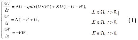
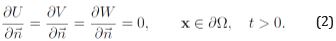
where we consider the chemotactic and hepatotactic coefficients, η and ρ, respectively, to be constant and positive. The parameter k represents the net growth of the tumor cell density. It is natural to assume homogeneous Neumann boundary condition as we assume that invasion takes place within an isolated system (see [2]). We consider for our numerical simulation
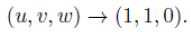
Tao and Winkler in [3] have demonstrated that whenever the initial data (U0, V0, W0) are regular fulfilling
U>o0, Wo ≤ 1 and K >η2/8, solution (U,V,W) converges asumptotically to the constant stationary solution (1, 1, 0) in the L∞(Ω). The GFDM has been recently proved to obtain highly accurate approximations to the solutions of nonlinear PDEs (see for instance [6,5,4]. The paper is organized as follows: in Section 2 we present the explicit formula of the GFDM and obtain the explicit scheme. In Section 3 we present numerical examples. In particular, the first example shows the convergence of the solution to the constant steady state (1, 1, 0), in accordance with the theory [3]. The second and third examples show that for an appropriate initial data the solution converges to (0, 0, ω), with ω arbitrary. Finally, we obtain some conclusions in Section 4.
GFD Scheme
As stated in the introduction, our objective is to derive a discretization of system (1) using the GDF explicit formulae. To do so, let us consider a bounded domain Ω ⊂ R2. Then,
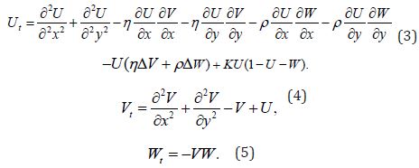
Therefore, system (1) reads as equations (3), (4) and (5) together with the nonnegative initial data

With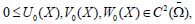 and the boundary conditions
The explicit formulae of the GFD explicit scheme can be seen in [4, 5, 6], although for the sake of completeness we reproduce below
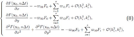
Where
For j = 0; 1; 2. The time derivative is approximated by
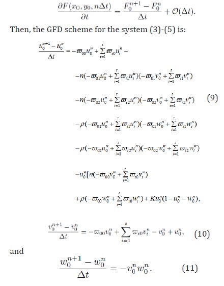
Then, the GFD scheme for the system (3)-(5) is:
Numerical Computations
We consider an irregular cloud of points see (Figure 1) modelling our in vitro domain. For all examples we denote by (u, v, w) the approximate solution given by the GFDM. For all numerical examples we use as time step Δt = 0.001 and, then, T (s) (total time) is calculated by nΔt .
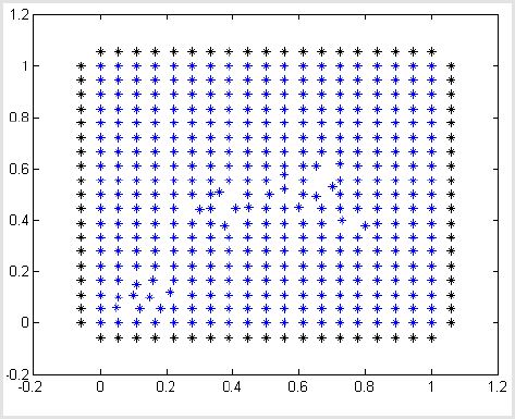
Figure 1: Irregular clouds of points.
Example 1
In this first example we solve numerically system given by (3)-
(5). We consider η = ρ = 0.5 and k =1.5 .
We take into account the following initial data:

As we have mentioned in Section 1, since the assumption κ > η2/8 is fulfilled, we expect to find convergence of the solution in the sense
In (Table 1)l∞ we present the of the approximate solution for different times. Figure 2 shows the different solutions at such times.
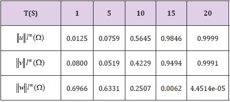
Table 1: Values of
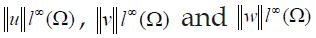 for different time values in the Example 1.
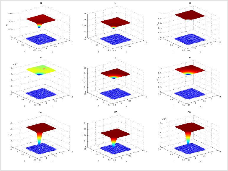
Figure 2: Approximate solution for 1, 10 and 20 seconds for Example 1.
Example 2
For this second case we also consider η = ρ = 0.5 and K =1.5 . As initial data we consider

Notice that W0 ≤ 1 does not hold. Then, the assumptions of [3] are not fulfilled. Table 2 shows the maximum value of the approximate solutions for different times [4]. Figure 3 shows the approximate solutions at 1, 10 and 20 seconds. We obtain convergence to the steady state (0, 0, 1). To the best of our knowledge no analytical proof of this convergence is known [5,6].

Figure 3: Approximate solution for 1, 10 and 20 seconds for Example 2.
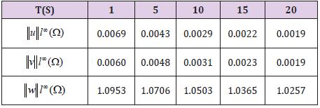
Table 2: Values of
 for different time values in the Example 2.
Example 3
Let us choose now η = 0.5 , ρ = 0.6 and K =1.5 . As initial data we consider the following
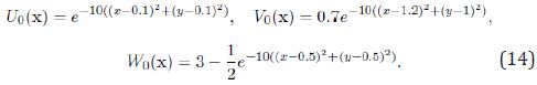
Table 3 shows the values norm of the approximate solutions. In this third case, where w(X ) ≤1 does not hold, we obtain convergence to the steady state (0, 0, 2.8109). In general, this means that solution to (1) converges to
(0,0,wˆ)
where wˆ is an arbitrary function (which seems to depend on ∫ΩW0(X )dX). Figure 4 shows the approximate solution of this third case. Note that we introduce the solutions at small times in order to capture the dynamical complexity of the model.

Table 3: Values of
 for different time
values in the Example 3.
for different time
values in the Example 3.

Figure 4: Approximate solution for 0, 0.1 and 1 seconds in Example 3.
Conclusion
We have derived the discretization of the chemotaxis-hypotaxis system (1) using a GFD scheme. The discrete solution obtained inherits the complicated dynamical behavior of the analytical solution. The Generalized Finite Difference Method solves this strongly coupled highly nonlinear parabolic-elliptic system efficiently and with high accuracy.
Acknowledgement
The authors acknowledge the support of the Escuela Technical Superior de Ingenious Industrials (UNED) of Spain, project 2019- IFC02, and of the University Polytechnical de Madrid (UPM) (Research groups 2019). This work is also partially support by the Project MTM2013-42907-P from MICINN (Spain).
References
- Chaplain MA J and Lolas G (2005) Mathematical modelling of cancer cell invasion of tissue: The role of the urokinase plasminogen activation system. Mathemat Models Methods Applied Sci 15(11): 1685-1734.
- Chaplain MA J, Lolas G (2006) Mathematical modelling of cancer cell inva- sion of tissue: Dynamic heterogeneity. Networks Heterogenous Media 1(3): 399-439.
- Tao Y, Winkler M (2015) Large time behavior in a multidimensional chemotaxis-haptotaxis model with slow signal diffusion. Siam J Math Anal 47(6): 4229-4250.
- Gavete ML, Vicente F, Gavete L, Urena F, Benito JJ (2019) Numerical sim- ulation in electrocardiology using an explicit Generalized Finite Difference Method. Biomed J Sci & Tech Res13(5).
- Benito JJ, Urena F, Gavete L (2001) Influence of several factors in the gener- alized finite difference method. Applied Mathemat Model 25: 1039-1053.
- Urena F, Gavete L, Garcia A, Benito JJ, Vargas AM (2019) Solving second order non-linear parabolic PDEs using generalized finite difference method (GFDM). J Comput Applied Mathemat 354: 221-241.
