 Research Article
Abstract
In this paper, we present a Robin-type nonoverlapping domain decomposition (DD) preconditioner, which is deduced from the renew equation of the Robin-Robin iteration method. The unknown variables to be solved in this preconditioned algebraic system are the Robin transmission data on the interface. Through choosing suitable parameter on each subdomain boundary and using the tool of energy estimate, for Raviart-Thomas vector field in three dimensions, we prove that the condition number of the preconditioned system is O (1), and the DD method is optimal. I prove the discrete extension theorem in H(div). Numerical results are given to illustrate the efficiency of our DD preconditioner.
Keywords: Finite Element Method; Robin-Type Domain Decomposition Method; Condition Number Estimate; Raviart-Thomas Vector Field; Optimal
Introduction
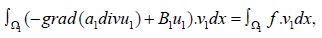
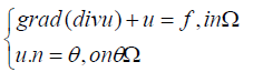
In this paper, we consider the following boundary value problem
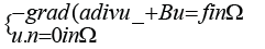
Given a bounded convex polyhedral domain Ω ⊂ R3 , we
introduce the boundary value problems where a∈L∞ (Ω) is a scalarvalued
positive function bounded away from zero, the coefficient
matrices  is symmetric uniformly positive definite with
 1 ≤ i j ≤ n and f ∈L2 (Ω)3 . The weak formulation of
problem (1.1), and the study of the Raviart-Thomas finite elements,
as well as our iterative method, require the introduction of an
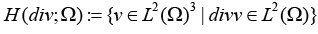
appropriate Hilbert space H(div;Ω) . It is given by
1 ≤ i j ≤ n and f ∈L2 (Ω)3 . The weak formulation of
problem (1.1), and the study of the Raviart-Thomas finite elements,
as well as our iterative method, require the introduction of an
appropriate Hilbert space H(div;Ω) . It is given by
which equipped with the inner product (.,.)div;Ω; and the
associated graph norm defined
by

The subspace of vectors in H(div;Ω)with vanishing normal component on ∂Ω is denoted by
H0(div;Ω) and it is the appropriate space for the variational formulation of (1.1):
Find u∈H0 (div;Ω) such that

where the bilinear form a(.,.) is given by

We associate an energy norm, defined by
 with
the bilinear form; our associations on the coefficients guarantee
that this norm is equivalent to the graph norm. Given a vector
u∈H(div;Ω), it is possible to define its normal component u. n
on the boundary [1].
with
the bilinear form; our associations on the coefficients guarantee
that this norm is equivalent to the graph norm. Given a vector
u∈H(div;Ω), it is possible to define its normal component u. n
on the boundary [1].
LEMMA 1.1.
Let Ω ⊂ R3 be Lipschitz continuous. Then, the operator
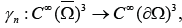 mapping a vector into its normal
component on the boundary, can be extended continuously to an
operator
mapping a vector into its normal
component on the boundary, can be extended continuously to an
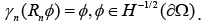
operator 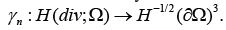 In addition, there exists
a continuous lifting operator
In addition, there exists
a continuous lifting operator 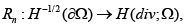 such that
 The following Green’s formula holds,
u∈H(div;Ω) and q∈H1(Ω),
The following Green’s formula holds,
u∈H(div;Ω) and q∈H1(Ω),
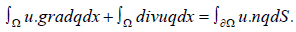
where the integral on the right hand side is understood as the
duality pairing between  . We consider finite
element discretization’s based on the Raviart-Thomas elements.
For triangulations made of tetrahedra, the local spaces on a generic
tetrahedron K are defined as
. We consider finite
element discretization’s based on the Raviart-Thomas elements.
For triangulations made of tetrahedra, the local spaces on a generic
tetrahedron K are defined as

where x is the position vector in Rn and Pk-1(K) is the space of homogeneous polynomials of
degree k−1 on K. A function u in Dk (K) is uniquely defined by the following degrees of freedom
for each face for each face f of K. For k > 1, we add
It can be proven that the following spaces are well-defined:

The corresponding interpolation operator is denoted by
 When there is no ambiguity,
we simply use the notations 
For the case k = 1, the elements of the local space have the simple form
It is immediate to check that the normal components of a vector in D1 (K) are constant on
each face f. These values
can be taken as the degrees of freedom.
The spaces H(curl;Ω) and H(div;Ω) , and special finite element approximations have been introduced to analyze equations such as (1.1); see [2]. In recent years, a considerable effort has been made to develop optimal or quasi-optimal, scalable preconditioners for these finite element approximations of problems in H(curl;Ω) and H(div;Ω) . Two-level overlapping Schwarz preconditioners for these spaces have been developed for two (see [3]) and three (see [4- 10]) dimensions, respectively. Multigrid and multilevel methods are considered in [11-28]. A few papers on the H(curl;Ω) case have proved optimality for a two-subdomain iterative sub structuring preconditioner, combined with Richardson’s method, for a lowfrequency approximation of time-harmonic Maxwell’s equations in three dimensions. In [19] the authors restrict themselves to two dimensions and develop an iterative sub structuring method for the problems in space H(curl;Ω) . In their work the condition number bound is independent of the number of substructures, it is developed locally for one substructure at a time and therefore insensitive to even large changes in the coefficients from one substructure to its neighbors.
Domain decomposition (DD) methods are important tools for solving partial differential equations, especially by parallel computers. In this paper, we shall study a class of nonoverlapping DD method, which is based on using Robin-Robin boundary conditions as transmission conditions on the subdomain interface. There is some iterative Robin-Robin DD method in the literature. This method was first proposed by Lions. Actually, the optimal transmission condition on the interface involves a nonlocal operator, which is not convenient to implement. So, adopting some local approximations to this operator becomes a useful way, which usually result in Robin-type boundary conditions. Some interesting Robin-type transmission conditions are considered in [21] for elliptic problem, and in [23] for the Helmholtz problem, respectively. Higher order approximation is also studied in [9], where they use the Pade approximates to localize the operator. However, the higher of approximation order, the more additional costs it has. The convergence was proved to be 1−O(h) in [16,25]. Then, in [29], Gander, Halpern, and Nataf improved it to be 1−O(h1/2 ) in the case of two subdomains. Later, Qin and Xu gave the convergence rate1−O(h1/2H1/2 ) in many subdomains. Later, Qin and Xu gave the convergence rate 1−O(h1/2H1/2 ) in many subdomain cases in [30], and further they used the Dirichlet-to-Neumann operator to prove that the convergence rate cannot be improved. A sharp convergent result is also obtained in [31-35]. For the case of arbitrary geometry interface, Liu also got the convergence rate to be 1−O(h1/2 ) in [22]. For the second-order Robin-type transmission condition, the convergence rate was improved to 1−O(h1/4 ) in [36]. Recently, for the two subdomain case, a new two-parameter Robin-Robin DD method was proposed by Chen, Xu, and Zhang in [37]. It is shown that the convergence rate is independent of the mesh size h without any additional computation. For the discontinuous coefficients problem, the convergence of the optimized Schwarz method was analyzed in [19] for the two subdomains case. In [30,31], the authors introduced some preconditioned systems of the optimized Schwarz method. In [29], the authors present a new Robin-type nonoverlapping domain decomposition (DD) preconditioner, and they have proved the preconditioner is optimal and scalable.
In this paper, we restrict ourselves to three dimensions and develop a preconditioner for equation (1.1). The preconditioner is induced from the Robin-Robin domain decomposition (DD) algorithm. We have proved that the condition bound is independent of h, so the method is optimal. To analyze the bound of the condition number, it has been necessary to obtain a continuous extension from the trace space ofH(div;Ω) into it, which has been constructed in [38]. The outline of this paper is as follows. In section 2, we will describe our Robin-Robin DD algorithm. In section 3, we will describe our preconditioner induced from the renew equation of the algorithm. In section 4, we will consider its corresponding condition number estimate. The implementation of this new DD algorithm will be discussed in section 5. Finally, some numerical results to verify our theoretical results will be given in the last section.
Model Problem and DD Algorithm
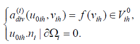
Problem (2.1) is equivalent to the following coupled problem, the equivalence can be proved
by considering the corresponding variational problems.
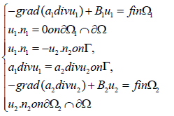
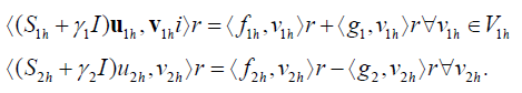
where the first transmission condition is chosen based on the fact that only the normal components of the finite element functions are continuous across the interelement boundaries, see [39,45]. The transmission conditions of (2.1) is equivalent to the following Robin-Robin boundary conditions:

where we allow γ1 ,γ2 to any positive constants such that 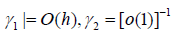
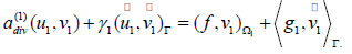
Let 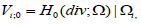 multiply the first equation of (2.1) by
 and integrate it
over Ω1, we get
by parts, with the Green’s formula, we get

Using the boundary condition (2.2), we get
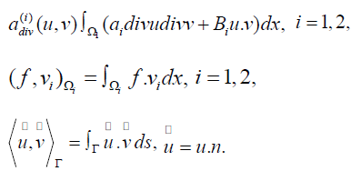
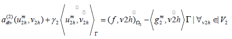
This way, we get the second variational problem on Ω2 :
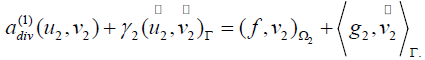
Where
Definition (The Robin-Robin DD method.) Given  on
Γ a serial version domain
on
Γ a serial version domain
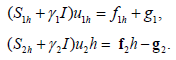
decomposition iteration consists the following five steps (m=0,1, ...):
a) Solve on Ω2 for 
b) Update the interface condition on Γ :
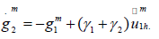
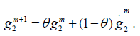
Get the next iterate by a relaxation:
The Preconditioner Induced from the DD Algorithm
Let  as follows:
Where  be the solution of the Dirichlet
problem:
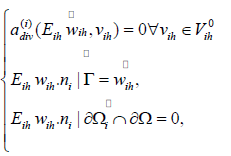
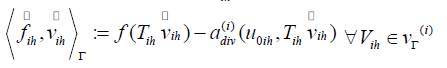
Define Sih to be a linear operator on VΓ which satisfies the following equations:
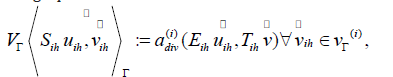
Where  is any extension such that
  Define fih satisfies
The definition of sih and fih is independent of the choice of
Tih for all 
Note that 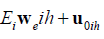 satisfying:
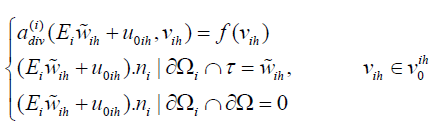
Based on Lax-Milgram theorem the solution of the problem is unique, i.e.
so that,

Therefore (2.3) and (2.4) are equivalent to
Because of the of the arbitrariness of vih, we obtain
The Robin-Robin Iteration is equivalent to
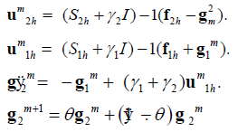
We induce that

Where
which shows that the renew equation of the Robin-Robin algorithm is a preconditioned Richarson iteration for the following equation:

where the preconditioned operator is Pr−1
We notice that
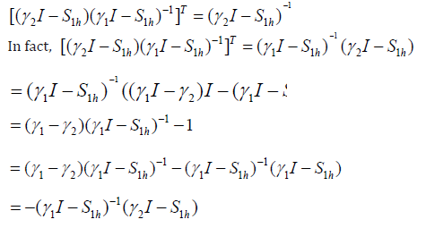
In the same way,

Thus, the operators G and Pr−1 are symmetric and Pr−1 is positive definite, G is also positive
definite will be proved later. Therefore we can use the preconditioned conjugate gradient (PCG)
method to solve the system.
The Condition Number Estimate
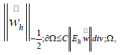
LEMMA 4.1. For the discrete harmonic extension operator Eh, we have (deduced from Theorem 2.5 in [32], or Lemma A.19 in [7])

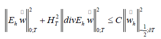
LEMMA 4.2: It holds that
Proof. The proof is similar to one given in [24, Lemma 4.3]. We will first prove the result for a
substructure T of unit diameter. Consider a Neumann problem:
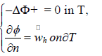
Here  is the derivative in the direction of the outward
normal of ∂T. Define an extension operator
is the derivative in the direction of the outward
normal of ∂T. Define an extension operator  where u = gradeφ, and ρh is the interpolant onto the Raviart-Thomas
space Xh(T), defined by the degrees of freedom of Xh are given
by the averages of the normal components over the faces of the
triangulation:
where u = gradeφ, and ρh is the interpolant onto the Raviart-Thomas
space Xh(T), defined by the degrees of freedom of Xh are given
by the averages of the normal components over the faces of the
triangulation:
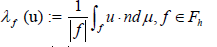
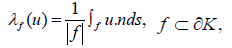
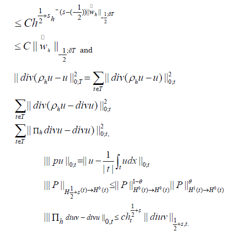
Where |f| is the area of the face f and the direction of the normal can be fixed arbitrarily for each face, we will show below that they {λf(u)} are well defined. Using the surjectivity of the map φ →∂φ onto Hs(T) and a regularity result given in [9, Corollary 23.3], we deduce
where ∈T is strictly positive and depends on T.
They {λf(u), f ∈ Fh} are well defined, since 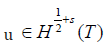 , with s > 0, then
Where 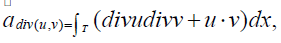 and Rn is the extension
of Lemma in [3].
and Rn is the extension
of Lemma in [3].
We find that
Where, 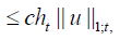
is the L2 projection onto the space of constant functions on each fine 
By interpolation theory, we have
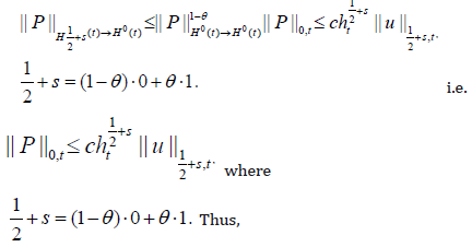
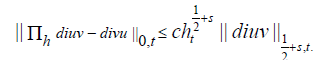
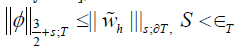
Employing an inverse inequality, we find that for s <∈T ,
therefore, 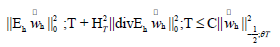 We now consider
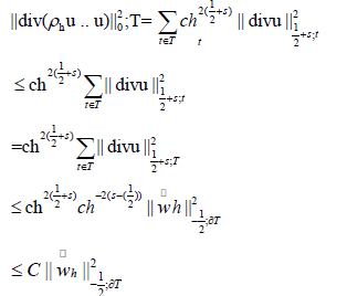
a substructure T of diameter H, obtained by dilation from a sub
structure of unit diameter. Using the previous result and by using a
scaling argument, we have
We now consider
a substructure T of diameter H, obtained by dilation from a sub
structure of unit diameter. Using the previous result and by using a
scaling argument, we have
Theorem 4.3.
Therefore
Theomem 4.4. It holds that

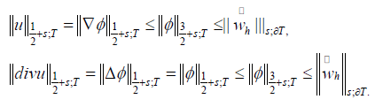
Proof we find that,
By inverse inequality, we have
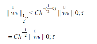
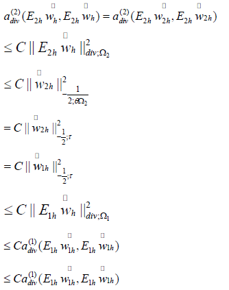
Combining (4.2), (4.3), and Lemma 4.2, we obtain
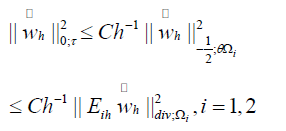
The final result is obtained by summing (4.4) over i = 1, 2
Theomem 4.5:
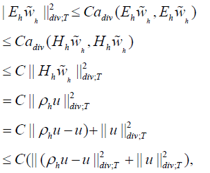
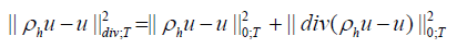
Proof. Based on Lemmas 4.1, 4.2, and the equivalence of the energy norm and graph norm, we
have,
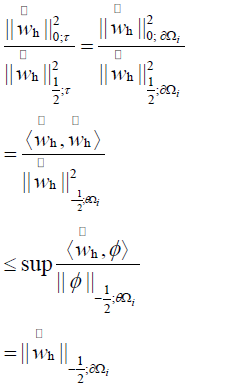
LEMMA 4.6. It holds that
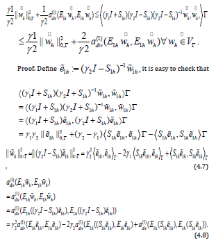
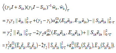
Based on the definitions in section 3, we have,
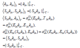
Combine (4.6), (4.7), (4.8) with (4.9), (4.10), (4.11), (4.12), we obtain,
Thus we have,
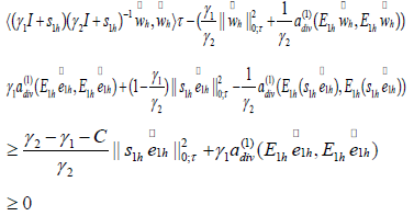
that is the left part of (4.5). On the other hand,
Thus,
Finally, based on the above inequality, we have
In the above inequality, we use the fact that  for sufficient small h. So
we have proved the right part of (4.5).
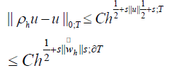
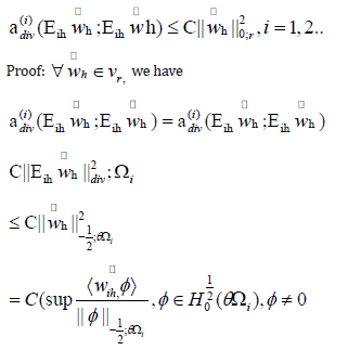
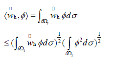
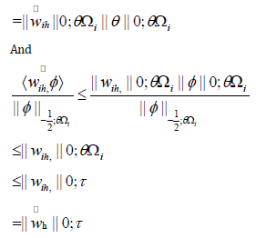
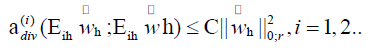
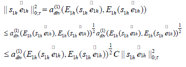
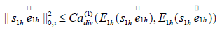
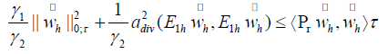
LEMMA 4.7. It holds that
Based on the definitions in section 3, we have,
Combine (4.14), (4.15), (4.16) with (4.17), (4.18), (4.19), (4,20), we obtain,
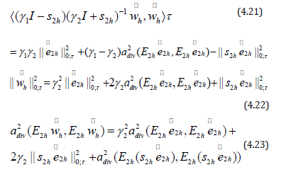
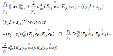
Applying Lemma 4.3 and (4.21), (4.22), (4.23), we have,
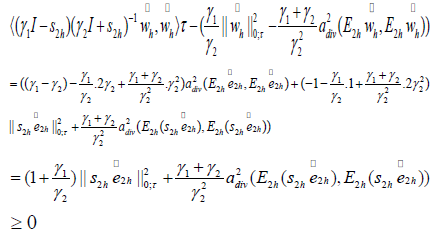
that is the left part of (4.13). On the other hand, we have
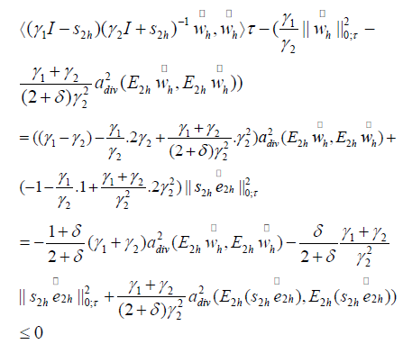
so we have proved the right part of (4.13). Based on Lemmas 4.6 and 4.7, we have Lemma 4.8.
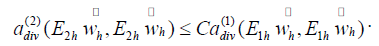
LEMMA 4.8. It holds that

Based on Lemmas 4.2, 4.3 and 4.8, we get the following main result of this paper.
THEOMEM 4.9. Assume that  then,
then,
Numerical Results
In this section, the convergence behavior of our new DD method will be checked by some numerical experiments. Consider the problem
Where,  and the function

The exact solution of this problem is  The domain Ω is divided
into 2 subdomains. We set the Robin parameters to be γ = h,2h
, γ2 = 50,100 which satisfy the condition of Theorem 4.9. The iteration stops when
The domain Ω is divided
into 2 subdomains. We set the Robin parameters to be γ = h,2h
, γ2 = 50,100 which satisfy the condition of Theorem 4.9. The iteration stops when 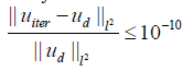 (Figures 1-4) and (Tables 1-4).
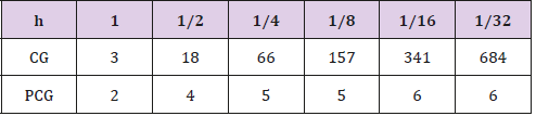
Table 1: Iterative number of γ1 = h and γ2 = 100.
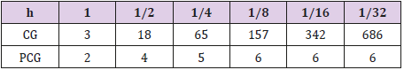
Table 2: Iterative number of γ1 = 2h and γ2 = 100.
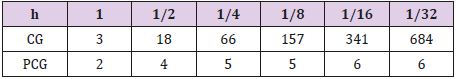
Table 3: Iterative number of γ1 = h and γ2 = 50.

Table 4: Iterative number of γ1 = 2h and γ2 = 50.
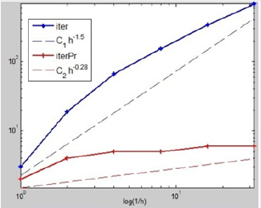
Figure 1: The figure describes the case of γ1 = h and γ2 = 100, where the ordinate values of these nodes on these polylines are iterative numbers which are the dates from Table 1, while the abscissa values of these nodes are the corresponding log(h). And the red ones describe the calculation processes with our precondition, while the blue ones describe the corresponding processes without our precondition. The dashed lines approximate the slopes of the corresponding polylines.
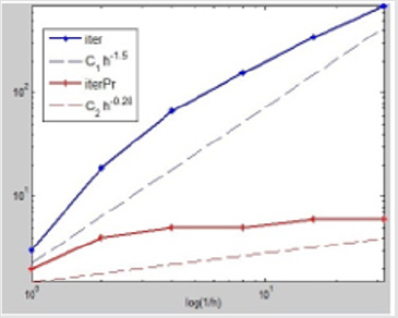
Figure 2: The figure describes the case of γ1 = 2h and γ2 = 100, where the ordinate values of these nodes on these polylines are iterative numbers which are the dates from Table 2, while the abscissa values of these nodes are the corresponding log(h). And the red ones describe the calculation processes with our precondition, while the blue ones describe the corresponding processes without our precondition. The dashed lines approximate the slopes of the corresponding polylines.

Figure 3: The figure describes the case of γ1 = h and γ2 = 50, where the ordinate values of these nodes on these polylines are iterative numbers which are the dates from Table 3, while the abscissa values of these nodes are the corresponding log(h). And the red ones describe the calculation processes with our precondition, while the blue ones describe the corresponding processes without our precondition. The dashed lines approximate the slopes of the corresponding polylines.
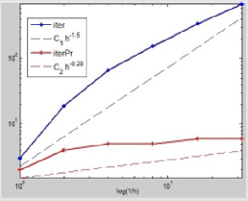
Figure 4: The figure describes the case of γ1 = 2h and γ2 = 50, where the ordinate values of these nodes on these polylines are iterative numbers which are the dates from Table 4, while the abscissa values of these nodes are the corresponding log(h). And the red ones describe the calculation processes with our precondition, while the blue ones describe the corresponding processes without our precondition. The dashed lines approximate the slopes of the corresponding polylines.
It is seen that as h decreases, the iteration numbers do not increase, which confirm our theoretical results reflect that our preconditioner is efficient and this preconditioned DD method is optimal.
Acknowledgement
We thank the anonymous referees who made many helpful comments and suggestions which lead to an improved presentation of this paper.
References
- Abdallah AB, Belgacem FB, Maday Y (2000) Mortaring the twodimensional “N´ed´elec” finite elements for the discretization of Maxwell equations. M2AN Math. Model. Numer Anal to appear.
- Adams RA (1975) Sobolev spaces, Academic Press New York, USA.
- Alonso A, Valli A (1996) Some remarks on the characterization of the space of tangential traces of H(rot; Ω) ant the construction of an extension operator, Manuscr. Math 89(1): 159-178.
- Alonso A, Valli A (1998) An optimal domain decomposition preconditioner for lowfrequency time-harmonic Maxwell equations, Math. Comp 68: 607-631.
- Amrouche C, Bernardi C, Dauge M, Girault V (1996) Vector potentials in three-dimensional nonsmooth domains, preprint R 96001, Laboratoire d’Analyse Num´erique, Universit´e Pierre et Marie Curic, Paris.
- Arnold DN, Falk RS, Winther R Multigrid in H(div) and H(curl). Numerische Mathematik 85(2): 197–217.
- Arnold DN, Falk RS, Winther R (1998) Multigrid preconditioning in H(div) on nonconvex polygons, Comput. Appl Math 17: 303-315.
- Arnold DN, Falk RS, Winther R (1997) Preconditioning in H(div) and applications. Math Comp 66: 957-984.
- Boubendir Y, Antoine X, Geuzaine C (2012) A quasi-optimal nonoverlapping domain de- composition algorithm for the Helmholtz equation J Comput Phys 231(2): 262-280.
- Brezzi F, Fortin M (1991) Mixed and hybrid finite element methods. Springer-Verlag, New York, USA.
- Chen W, Liu Y, Xu XA Robust Domain decomposition method for the Helmholtz Equation with High Wave Number, submitted.
- Chen W, Xu X, Zhang S (2014) On the optimal convergence rate of a Robin-Robin domain decomposition method. J Comp Math 32(4): 456- 475.
- Costabel M (1990) A remark on the regularity of solutions of Maxwell’s equations on Lipschitz domains. Math Meth Appl Sci 12: 365-368.
- Dauge M (1988) Elliptic Boundary Value Problems on Corner Domains. Springer-Verlag, Berlin.
- Dautray R, Lions JL (1988) Mathematical analysis and numerical methods for science and technology. Springer-Verlag, New York, USA.
- Deng Q (2003) A nonoverlapping domain decomposition method for nonconforming finite element problems. Comm Pure Appl Anal 2(3): 295-306.
- Douglas J, Huang Jr, Huang CS (1998) Accelerated domain decomposition iterative pro- cedures for mixed methods based on Robin transmission conditions. Calcolo 35(3): 131-147.
- Douglas J, Huang Jr, Huang CS (1997) An accelerated domain decomposition procedure based on Robin transmission conditions. BIT 37(3): 678-686.
- Dubois O, Lui SH (2009) Convergence estimates for an optimized Schwarz method for PDEs with discontinuous coefficients. Numer Algorithms 51(1): 115-131.
- Ernst OG, Gander MJ (2012) Why it is difficult to solve Helmholtz problems with classical iterative methods, in Numerical Analysis of Mutiscal problems. I Graham, T Hou, O Lakkis, R Scheichl (eds.). Lect Notes Comput Sci Eng Springer, Heidelberg, 83: 325- 363.
- Gander MJ (2006) Optimized Schwarz methods. SIAM J Numer Anal 44(2): 699-731.
- Gander MJ, Halpern L, Nataf F (2001) Optimized Schwarz methods, in Proceedings of the 12th International Conference on Domain Decomposition Methods. In: T Chan, T Kako, H Kawarada, O Pironneau (Eds.), Chiba, Japan, Domain Decomposition Press, Bergen, Norway, p. 15-18.
- Gander MJ, Magoules F, Nataf F (2002) Optimized Schwarz methods without overlap for the Helmholtz equation. SIAM J Sci Comput 24(1): 38-60.
- Girault V, Raviart PA (1986) Finite element methods for Navier-Stokes equations, Springer- Verlag, New York, USA.
- Guo W, Hou LS (2003) Generalizations and accelerations of Lions’ nonoverlapping domain decomposition method for linear elliptic PDE, SIAM J. Numer Anal 41(6): 2056-2080.
- Hiptmair R, Toselli A (2000) Overlapping and multilevel Schwarz methods for vector valued elliptic problems in three dimensions. Parallel solution of PDEs, IMA Volumes in Mathematics and its Applications. Springer-Verlag, Berlin, pp. 181-208.
- Hiptmair R (1997) Multigrid method for H(div) in three dimensions. Electron Trans Numer Anal 6: 133-152.
- Hiptmair R (1998) Multigrid method for Maxwell’s equations. SIAM J Numer Anal 36(1): 204-225.
- Liu Y, Xu XA (2014) Robin-type domain decomposition method with redblack partition. J Numer Anal 52(5): 2381-2399.
- Loisel S (2013) Condition number estimates for the nonoverlapping optimized Schwarz method and the 2-Lagrange multiplier method for general domains and cross points. SIAM J Numer Anal 51 (6): 3062- 3083.
- Lui SH (2009) A Lions non-overlapping domain decomposition method for domains with an arbitrary interface. IMA J Numer Anal 29(2): 332- 349.
- Makridakis CG, Monk P (1995) Time-discrete finite element schemes for Maxwell’s equations, RAIRO M 2AN 29(2): 171-197.
- Monk P (1992) Analysis of a finit element method for Maxwell’s equations. SIAM J Numer Anal 29(3): 714-729.
- Nedelec JC (1980) Mixed finite elements in 3, Number. Math 35(3): 315- 341.
- Qin L, Xu X (2006) On a parallel Robin-type nonoverlapping domain decomposition method, SIAM J Number Anal 44(6): 2539-2558.
- Quarteroni A, Valli A (1994) Numerical approximation of partial differential equations, Springer-Verlag, Berlin.
- Quarteroni A, Landriani GS, Valli A (1991) Coupling of viscous and inviscid Stokes equations via a domain decomposition method for finite elements 59(1): 831-859.
- Toselli A (1999) Domain decomposition methods for vector field problems, Ph.D. thesis, Courant Institute of Mathematical Sciences, Technical Report 785, Department of Computer Science, Courant Institute of Mathmatical Sciences, New York University, USA.
- Toselli A (2000) Overlapping Schwarz methods for Maxwell’s equations in three dimensions, Nu- mer Math, to appear 86(4): 733-752.
- Toselli A, Widlund O (2005) Domain Decomposition Methods-Algorithms and Theory, Springer Ser. Comput. Math. 34, Springer-Verlag, Berlin.
- Toselli A, Widlund OB, Wohlmuth BI (1998) An iterative Substructuring Method for Maxwell’s Equations in Two Dimensions, Technical Report 768, Department of Computer Science, Courant institute, New York university, New York, NY, USA.
- Valli A (1996) Orthogonal decompositions of (L2(Ω))3, preprint UTM 493, Dipartimento di Matematica, Universit´a di Trento.
- Wohlmuth BI, Toselli A, Widlund OB (2000) An Iterative substructuring method for Raviant- Thomas vector fields in three dimensions. SIAM J Numer Anal 37(5): 1657-1676.
- Xu J, Zou J (1998) Some nonoverlapping domain decomposition methods, SIAM Rev 40(4): 857-914.
- Xu X, Qin L (2010) Spectral analysis of Dirichlet-Neumann operators and optimized Schwarz methods with Robin transmission conditions. SIAM J Numer Anal 47(6): 4540-4568.
