info@biomedres.us
+1 (502) 904-2126
One Westbrook Corporate Center, Suite 300, Westchester, IL 60154, USA
Site Map
Received: October 29, 2018; Published: November 05, 2018
*Corresponding author: Sergey Belyakin, Physics of Faculty, Department of General physics, Moscow 119192, Russia
DOI: 10.26717/BJSTR.2018.10.002005
Autonomous hyperbolic attractors were introduced: by Smale and Anosov, Alekseev, Williams, Sinai, Ruelle, and other Neuhausen, about 70 years ago. Traditional examples of uniformly hyperbolic attractors are discrete-time geometric models such as the Smale - Williams attractor or the Plykin attractor presented in Figure 1 [1]. Initially, they were expected to be adequate for many real-world situations of chaotic behavior, such as hydrodynamic turbulence, etc. As time passed, it became clear that the early hyperbolic theory was too narrow to include most chaotic systems of interest to applications. So, the efforts of mathematicians were redirected to generalizations of the theory corresponding to wider classes of systems. For example, we developed the notion of nonuniform hyperbolic attractors, partially hyperbolic systems, quasihyperbolicity or singular hyperbolic attractor, quasi-attractor, etc. Uniformly hyperbolic attractor is presented in Figure 2, is an attractive object in the phase space of a dissipative dynamic system consisting exclusively of saddle trajectories.
Figure 1: The evolution of a hyperbolic strange attractor of Plykin-like attractor of Smale - Williams.

Figure 2: Stable (A < 0) (yellow) and unstable (A > 0) (blue) manifolds represent the same dimension for all trajectories on a strange attractor, (red line) a small neighborhood of unstable equilibrium (A < 0).

Their stable and unstable manifolds have the same dimension for all trajectories on the attractor; they should not touch; only intersections with non-zero angles are allowed. The hyperbolic nature of the attractors can be verified using the cone criterion. The Figure 3 below shows this for a discrete time system (iterated map). Cones of expanding and compressing infinitesimal perturbation vectors must exist at each point of the region containing the attractor, which smoothly depends on the position. The image of the expanding cone shall be placed inside the expanding cone at the point of the image, and the prototype of the connecting cone shall be placed inside the dosing cone at the point of Providence. For flows, the same considerations apply in terms of the Poan- care map. Geometric constructions of hyperbolic attractors of the Smale-Williams Attractor. The mathematical theory of chaos, based on a strict axiomatic Foundation, deals with strange attractors of hyperbolic type Figure 4. In such an attractor, all orbits belonging to it in the phase space of the saddle system, with stable and unstable varieties (invariant sets composed of trajectories approaching the original in forward or reverse time) intersect transversally, i.e. without touching.
Figure 3: The cone criterion for the system with discrete time (the cones of the expanding and compressing of infinitesimal perturbation vectors, the iterated map).

Figure 4: Evolution of a strange hyperbolic attractor

Unfortunately, known physical systems, such as simple chaos generators, nonlinear oscillators with periodic action and others, do not belong to the class of systems with hyperbolic attractors. Chaos in them is usually associated with the so-called quasi-tractor, which, along with chaotic trajectories includes stable orbits of a large period (not distinguishable in solving equations on the computer because of the narrowness of the regions of attraction). Hyperbolic strange attractors are robust (structurally stable). This means the insensitivity of the nature of movements and the relative position of trajectories in the phase space with respect to the variation of the equations of the system. In contrast to the hyperbolic attractor, quasi-attractors are characterized by a sensitive dependence of the dynamic's details on the parameters. This is obviously undesirable for potential applications of chaos, such as communication systems, signal masking, etc. Thus, from both a fundamental and applied point of view, it is interesting to implement hyperbolic chaos in physical systems.
In textbooks and monographs on nonlinear dynamics, examples of hyperbolic attractors are presented by abstract constructions. For example, the Smale-Williams attractor is constructed to map a three-dimensional space into itself defined by the following procedure. Consider an area in the form of a torus, stretch it in length, fold it in half and enclose it in the original torus, as shown in the figure. Each next iteration doubles the number of" turns". An object that is obtained within many iterations is called the Smale - Williams solenoid. Its transverse structure has the form of a Cantor set. If we introduce the angular coordinate of the depicting point q, then on successive iterations it obviously obeys the Bernoulli map qn+1={2qn}. In the remaining two directions, the phase volume element undergoes compression. Therefore, a system of coupled non - autonomous generators seems to be a suitable candidate from the point of view of the implementation of the Smale-Williams attractor. Consider a one-dimensional map: xn+1={2xn}, where the braces represent the fractional part of the number. Its graph and diagram illustrating the dynamics over several iterations is shown in Figure 5. It is convenient to represent the variable x in the binary notation, with the digit 0 at the first position after the dividing point corresponds to the location of the representing point in the left, and 1 - in the right half of the unit interval. Let, for example, one step of evolution in time is that the sequence of zeros and ones is shifted to the left by one position, and the figure that appears on the left side of the dividing point is discarded, and so on. This transformation of the binary sequence, consisting in the shift of all characters to one position, called the Bernoulli shift.
Figure 5: The one-dimensional map xn+1={2xn}, where the braces denote the fractional part of the number, the graph and the diagram illustrate the dynamics over several iterations.

Figure 6: Non-Autonomous oscillatory system based on two oscillators with characteristic frequencies ω0 and 2ω0.

Let's set the initial state as a random sequence of numbers, for example, obtained by tossing a coin, according to the rule eagle - 0, tails - 1: x0 = 0.0101101... Then, during iterations, the depicting point will visit the left or right half of the unit interval exactly following our random sequence, thus causing chaos. The small perturbation of the initial condition is doubled in one step of iterations. Therefore, the Lyapunov exponent for this map is ln 2 = 0.693. How to implement dynamics corresponding to the Bernoulli map in a physical system. Let us turn to the flowchart shown in Figure 6. This is a non-Autonomous oscillatory system built based on two oscillators with characteristic frequencies ω0 and 2ω0. The parameter controlling the excitation of one and the other oscillator slowly changes in time in the counterphase with a period T, which is an integer number of periods of the fundamental frequency: T = 2πN/ω0. Thus, one or the other generator is excited in turn. The influence of the first generator on the second one is made through a nonlinear quadratic element.
The generated second harmonic serves as a seed when the ssecond generator is excited. In turn, the second generator acts on the first through a nonlinear element, which mixes the incoming signal and the auxiliary reference signal at a frequency «0. In this case, a component appears at the difference frequency. It resonates with the first generator and serves as a seed when it starts generating. Both generators, as it were, in turn transmit excitation to one another. Let us explain why the scheme functions as a generator of chaos. Suppose that at the stage of generation of the first oscillator oscillations have some phase φ. The signal at the output of the coupling element cosntains a second harmonic, and its phase 2φ is transmitted to the second oscillator when it starts to generate. Due to the mixing with the reference signal on the second coupling element, the doubled phase is transmitted to the initial frequency range, so that when the first oscillator is excited, at the next stage of generation, it will receive a phase 2φ. At successive excitation stages of the first generator for its phase normalized to 2π, Θ= φ/2π, the Bernoulli map will be valid: Θn+1= {2Θ n}. To observe the described mechanism numerically, we consider a system of equations (1), two Van - Der - Pol oscillators with variable coefficients:

For Figure 7 the time dependence of the variables x and y in this system, performing a chaotic motion in the relay transmission of excitation from one oscillator to another, is shown. The graph is based on the results of the numerical solution of the equations at ω0 = 2π, T = 10, A = 3, ε = 0.5.
Figure 7: The time dependence of the variables x and y in this system, performing a chaotic motion in the relay transmission of excitation from one oscillator to another at ω0 = 2π, T = 10, A = 3, ε= 0.5, is shown.

Figure 8: The time dependence of the variables x and y in this system, performing a chaotic motion in the relay transmission of excitation from one oscillator to another at ω0 = 2π, T = 6, A = 5, ε= 0.5, is shown.

For Figure 8 the time dependence of the variables x and y in this system, performing a chaotic motion in the relay transmission of excitation from one oscillator to another, is shown. The graph is based on the results of the numerical solution of the equations at ω0 = 2π, T = 6, A = 5, ε = 0.5. Chaos manifests itself in the random walk of the highs and lows of filling relative to the envelope. Below is a diagram of the empirical mapping for the phase of the first oscillator in the middle of the excitation stages. On chart Figure 9, the points (Θn, Θn+1 ) are postponed for a sufficiently large number of periods T. So, we obtain a map that, despite the presence of some deformations, is topologically equivalent to the Bernoulli map ΘnΘ1 = {20n}. In fact, if we vary the initial phase so that the depicting point once bypassed the full circle, the point-image will make a two-time circumference. This is expressed in the fact that the graph has two branches, located in the same way as in the first figure at the beginning of this page. The correspondence with the Bernoulli's classical map becomes better when the ratio of periods increases N. The last Figure 10 shows a graph of the dependence of the higher exponent of the Lyapunov (A), for a system of coupled nonautonomous Van - Der - Pol oscillators on the amplitude of the slow modulation a, with the period taken as a unit of time T.
Figure 9: Pending points (Θn, Θn+1) for a sufficiently large number of periods T.

Figure 10: A graph of the dependence of the higher Lyapunov exponent (A) for a system of coupled nonautonomous Van - der - Pol oscillators on the amplitude of the slow modulation A for fixed other parameters is presented.

As you can see, in a wide range of parameter Lyapunov exponent remains almost constant and approximately equal to ln2 = 0.693, corresponding to the Bernoulli map. At small A the correspondence disappears - the Lyapunov exponent becomes noticeably smaller.
Cardiovascular diseases (CVD) are responsible for 4 million deaths in Europe each year and cause a decline in life expectancy of 30%. The main group of CVD is associated with disorders of normal heart rhythm (cardiac arrhythmias). The heart rate is not a strictly periodic process, since the heart muscle is not an isolated system. In a healthy state, the heart always responds to physical activity, respiratory rhythm, etc. [2]. Moreover, periodic excitation of sthe heart indicates pathology, and strictly regular contractions of the heart can lead to its sudden stop and, therefore, to the death of the body (see, for example, [3-5]). However, arrhythmias are a completely different kind of aperiodic behavior of the heart. In this case, the heart muscle is no longer amenable to simple control with the help of incoming impulses. Arrhythmia - is any heart rhythm that differs from the normal sinus rhythm by changes in the frequency and regularity of the source of excitation of the heart, as well as by a violation of the conduction of pulses.
From this point of view, arrhythmias can be divided into three large groups. One of them-arrhythmias due to violation of the passage of impulses. For example, atrioventricular blockade of the heart may be characterized by abnormal coordination between the atrial and ventricular rhythms, leading to an extension of the interval between atrial and ventricular contractions (AV-blockade of 1 degree), an increase in the number of atrial contractions compared to the number of ventricular contractions due to the blocked conduct of some of the atrial beats (AV-blockade of 2 degree) or a complete lack of coordination between atrial and ventricular rhythms (AV-blockade of 3 degree). Such an AV blockade, as the rhythms of Venkebah, due to the increase in the interval between contractions of the Atria and ventricles, leading to the loss of one of the ventricular beats. Another group is arrhythmias that occur as a result of impaired impulse formation.
sFor example, irregular excitation of Central cells of ACS leads to such types of disorders as sinus bradycardia (low heart rate), while the frequency of excitations and contractions of the heart can be determined by the activity of the second or third order rhythm drivers, and tachycardia (high rate of contractions) associated with the generation of heart rate by parasitic high-frequency sources. Arrhythmia due to competition ACS and spurious (ectopic), the leading centre emerged from a group of contractile cardiomyocytes, for the reference rate, is called Parasitology. The third group of abnormalities - arrhythmia due to combination of violations. All types of cardiac arrhythmias can also occur in the absence of anatomically expressed changes in the myocardium in practically healthy people, and in this case, they are called functional, unlike pathological disorders that occur with organic changes in the heart (see [6]). The theory of dynamic systems describes many processes inherent in active media, including some types of arrhythmias [7]. Since arrhythmias are caused by certain disorders in the heart muscle and, therefore, are pathological conditions, the modeling of such systems is of great practical interest and can bring closer to the solution of the question of the possibility of controlling their behavior through external influences. This, in turn, allows us to come close to the problem of soft withdrawal of active systems from the state of developed space-time chaos characterizing some types of pathologies [8-10].
For the first time an electronic device is implemented Figure 11, which is an Autonomous dynamic system with a hyperbolic attractor of the Smale - Williams type. The experimental study of the laboratory model of the hyperbolic chaos generator is carried out and the correspondence of the observed dynamics to the results of numerical calculations and circuit simulation in the software environment Multisim (together with lab. SF-6) Figure 12 [11]. For Figure 11 the scheme of the analog device which dynamics is described by equations is shown:
Figure 11: Scheme of the device, the dynamics of which is described by a system of equations (1) with coefficients and parameters MS, Dynamic variables x, y, z, v corresponds to the voltages on capacitors C1, C2, C3, C4, measured in decivolts.

Figure 12: Experimental study of the laboratory model of the hyperbolic chaos generator and demonstrated compliance of the observed dynamics with the results of numerical calculations and circuit simulation in the Multisim software environment.

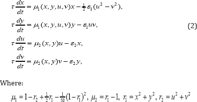
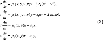
Each of the four dynamic variables x, y, u, v is associated with a fragment of the circuit, which is an integrator based on the operational amplifier (respectively, U1, U2, U3, U4), capacitance (C1, C2, C3, C4) and resistance (R13, R14, R16, R17). The actual values of x, y, u, v correspond to the voltages on capacitors C1, C2, C3 and C4, respectively. Constant with the dimension of time is defined in terms of capacitance and resistance, and if specified in the diagram the values is milliseconds Figure13. For the presented scheme, the coupling coefficients are. The system (2) is closed and Autonomous. Add to the system the external periodic action f = Asinwt, and the resulting system becomes non-Autonomous (3).
Figure 13: Photos from the oscilloscope screen of the hyperbolic attractor portrait are presented: time dependences (x(t), y(t), u(t), v(t)) at the top, phase portraits ((x,y), (x,v) and Fourier spectra (x, u) at the bottom.

Lyapunov exponents (X (a, «)) of equation (3) are presented in Figure14.
In Figure 14-18, various variants of system behavior (3), which can be used in the presentation of various heart failure, are considered. In Figures 19-20, presents real ECG data that can be used to study and predict the behavior of heart failure current models. Based on classical models of Duffing and Lorentz [1,11,12], current models are used to represent various behaviors of heart failure.
Figure 14: Lyapunov exponents (λ (a, ω)) of the equation (3).

Figure 15: A portrait of a hyperbolic attractor at A = 0 is presented: above the time dependence (x(t)) and phase portraits (x, x), (x, y) and (x, v), below the time dependence (x(t)) and phase portraits ((x, y), (xn+1, xn), (xn+1 - xn, xn+1 + xn)) and Fourier (x) spectrum.

Figure 16: A portrait of a hyperbolic attractor is presented for A = 1, m = n: above the time dependence (x(t)) and phase portraits (x, x), (x, y) and (x, v), below the time dependence (x(t)) and phase portraits ((x, y), (x , xn), (x - xn, xn+1 + xn)) and Fourier (x) spectrum.

Figure 17: A portrait of a hyperbolic attractor is presented for A = 2, ω = n: above the time dependence (x(t)) and phase portraits (x, x), (x, y) and (x, v), below the time dependence (x(t)) and phase portraits ((x, y), (x , xn), (x - xn, xn+1 + xn)) and Fourier (x) spectrum.

Figure 18: A portrait of a hyperbolic attractor is presented for A = 4, ω = n: above the time dependence (x(t)) and phase portraits (x, x), (x, y) and (x, v), below the time dependence (x(t)) and phase portraits ((x, y), (xn+1, xn), (xn+1 - xn, xn+1 + xn)) and Fourier (x) spectrum.

Figure 19: ECG Belyakin S.T. conducted during a medical examination of the clinic MSU them. M. V. Lomonosov. 17.08.2017.

Figure 20: ECG 12-introductory, 24-year-old black female patient with sickle cell anemia, renal failure, and hyperparathyroidism. The level of calcium in the blood serum of the patient was 7 mg / DL, and potassium level of 6.5mEq / L. The ECG shows prolongation of the ST segment and the QTU interval (given in V5 and V6). And hypokalemia and hypomagnesemia, expressed by lengthening of QTU and alternative QTU (indicated by arrows); B - C - D are represented by rhythmic stripes of the same patient, showing tachycardia - (dependent QTU) and alternative tachycardia indications are indicated in [12].


