info@biomedres.us
+1 (502) 904-2126
One Westbrook Corporate Center, Suite 300, Westchester, IL 60154, USA
Site Map

Received: September 08, 2018; Published: September 25, 2018;
*Corresponding author: John E Kolassa, Department of Statistics and Biostatistics, Rutgers, the State University of New Jersey, Hill Center 501,110 Frelinghuysen Rd, Piscataway NJ 08854, USA
DOI: 10.26717/BJSTR.2018.09.001783


This paper presents a modified chi-square approximation to the distribution of test statistics arising from multivariate ranked data. The modification arises from an improvement to the estimated variance matrix of the responses and from corrections for continuity and skewness and kurtosis of the rank sum statistics.
Kawaguchi et al. consider tests of equality of means for multivariate responses, in the presence of covariates, stratification, and tied and missing data. They propose inference based on approximating the joint distribution of Wilcoxon rank sum statistics as multivariate normal, with an estimated covariance matrix. They present a test statistic that may be expressed as a quadratic form of Wilcoxon rank sum statistics, with the variance-covariance matrix estimated using methods derived by Davis and Quade; they also apply this multivariate normal approximation to derive univariate confidence intervals. In this paper, we examine the effect of some alternative variance matrix estimates and also investigate the usefulness of the approximation of Yarnold, correcting for discreteness, skewness and kurtosis [1-3].
Consider subjects on which two or more variables (Yj1 . . . , YjD) are observed on each of M + N subjects, here indexed by j. Assume that the collection of vectors

are independent, with a continuous distribution. Suppose that these sub- jects are divided into two groups, with subjects j = 1, . . ., M in the first group and subjects j = M + 1, . . . , M + N in the second group. This paper presents distributional results of use in certain hypothesis tests involving the process generating these data. Under both the null and alternative hypothesis, assume that the collection of vectors {(Yj1 . . . , YjD), j ≤M } have the same distribution, and that the collection of vectors {(Yj1 . . . , YjD), j ≥ M} have the same distribution, and in the entirety of this paper, the null hypothesis specifies that these two common distributions are the same. The alternative hypothesis is that that the common distribution of the vectors in {(j1 . . . , YjD), j ≤ M} is different from the common distribution of {(j1 . . . , YjD), j > M}. Furthermore, alternatives of interest are those for which values of one group are systematically higher than those of another. For example, Kolassa and Seifu apply this to two groups of cancer patients (early vs. advanced) and look for differences in PSA and Gleason score between these two groups [4]. As noted above, we test the null hypothesis that all of these vectors are identically distributed, vs. the alternative hypothesis that those vectors for which j ≤ M have a distribution different from that for which j > M , and again, we choose a test statistic expected to have power when there exists k for which the distribution of Yjk, with j ≤ M , is stochastically larger or smaller than that of Yjk with j > M.
Testing in this manuscript will be performed by constructing univariate Mann-Whitney-Wilcoxon statistics for each variable and combining these statistics into a quadratic form. Let

Otherwise the two-sample univariate Mann-Whitney statistics for testing the null hypothesis that the distribution of Yjk, for j ≤ M, is the same as that of Yjk, for j > M . As above, j indexes subject, and k indexes variable, and i represents a second subject index, when pairs of subjects must be considered at the same time. The expectations and marginal variances of Tk under the null hypothesis are NM/2 and NM (N + M + 1)/12 respectively. Let σkl be the covariance between Tk and T|. One might test the equality of distribution of (Yj1 . . . , YjD), for j≤M , and that of Yj1, . . . , YjD, for j > M, by rejecting the null hypothesis for large values of

where ϭkl is the entry in row k and column l of the matrix inverse of the variance-covariance matrix given by ϭkl. Again, k indexes variable, and l is a second variable index used when pairs of variables must be considered.
Covariances between components of
T = (T1....Td ) (4)
must be estimated empirically. In a context generalized by the presence of missing and tied data, Kawaguchi et al. estimate the variance of T using a method originating with Davis and Quade. Kawaguchi and Koch apply these methods to crossover studies [1,2,5].
Many statistics for testing multivariate statistical hypotheses can be expressed as quadratic forms of vectors of (often dependent) means of random quantities, where the matrix defining the quadratic form is the inverse of the variance-covariance matrix of entries in this vector. Such statistics are of the form (3). Constructing a test from such a quadratic form requires the approximation of tail probabilities for these quadratic forms. The first subsection will address approximation of probabilities associated with Wc when ϭij are known exactly; the next subsection will address the added complexity when ϭij are estimated.
Let w be the observed value of W. Represent the critical region for the test of the null and alternative hypotheses of 1.1 as c, the compliment of the set

for W as in (3). Were T of (4) to have arisen as the mean of independent and identically distributed vectors confined to a unit lattice, one might use the approximation of Yarnold to adjust for discreteness, skewness, and variance [3]. Discreteness is adjusted for by examining the difference between V (ω), the volume of the ellipse ω and N (w), the number of points T in this ellipse. Skewness and kurtosis are adjusted for using terms calculated from multivariate third and fourth cumulants. Let Kijk and Kijk be joint third and fourth order cumulants of T. Let
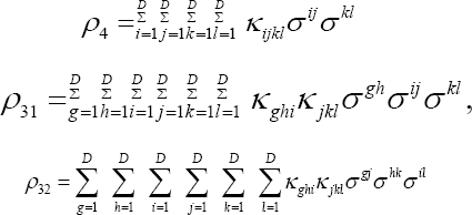
be the invariant multivariate kurtosis and skewness measures proposed by McCullagh and Cox and Mardia, and let δ1 = ρ4/8 and
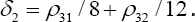
The approximation to the tail probability that corrects the γ2 approximation for continuity, skewness, and kurtosis is
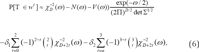
where Σ is the matrix with ϭij in row i and column j [6,7]. When (T1, . . . , TD) arises as the sum of n independent and identically- distributed random vectors, then δ1 and δ2 are of size O(1/n), and consequently so are the terms they multiply. Yarnold, citing Esseen, notes that the term adjusting for discreteness is of size O(n-D/(1+D)) and omits another correction for discreteness no larger than O(n-1) [3,8]. This omitted correction is not demonstrated to be smaller than the included term of size O(n-1).
We apply (6) in a situation in which (T1, . . . , TD) is not the sum of n independent and identically-distributed random vectors; specifically, we examine the case in which these are marginal Mann- Whitney statistics. Does shows that univariate Edgeworth series hold in such cases, to order O(1/n), without continuity correction [9]. Continuity corrections are of size o(1/n) in this case, rather than O(n-1/2), because, after standardizing to unit variance, lattice spacings for univariate Mann-Whitney statistics are O(n-3/2) rather than O(n-1/2), as they are for sums of independent and identically distributed random variables. Asymptotic orders of corrections for multivariate Mann-Whitney statistics are unknown, but likely to be also o(n-1).
Kawaguchi et al. present an estimator for the variance- covariance matrix of T, in the presence of a mechanism that potentially allows missing values in the raw data (1). Their distributional approximations use the approach of Davis and Quade [2]. In order to place our result in the proper context, we adopt the notation of Kawaguchi et al. [1]. The generic data item is denoted above in �1 by Yjk, for j representing subject and k representing variable measured on subject j. Refer to subjects with j ≤ M as being in group 1, and to subjects with j > M as being in group 2. Let nj be the number of subjects in the same group as subject j. Define the array element Vjjk for subjects j and jj, and response variable k, to be 1 if j and j’ are in different groups, and 0 otherwise. Let Ujjk be 1 if Vjjk is 1, and the value of response k in group 2 exceeds the value in group 1. Let Ujjk be 0 if Vjjk is 0, or if the value of response k in group 1 exceeds the value in group 2. Then, in the notation of �,
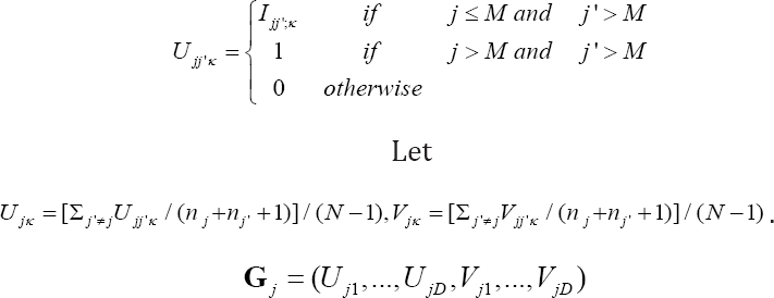
Otherwise, let G be the mean of vectors Gj and let s be the conventional sample variance-covariance matrix of the vectors Gj Then S= 4s/N is the estimated variance matrix for G under
the randomization distribution.  The propagation of errors method leads one to estimate the variance matrix of T by

for  where I is the identity matrix with number of rows and columns given by the subscript.
Kawaguchi et al. note that estimation of I extends easily to the case of independent strata, by adding estimates of this variance-covariance matrix calculated on a per-stratum basis [1]. Their treatment extends to estimation of the variance-covariance structure of response variables and covariates and from this joint structure, to a conditional structure adjusting responses for covariates. In the absence of tied and missing observations, the final D components of G in (7) are fixed, and the variances of the first components are known to be mn(m + n+1)/12, without the need for estimation. Let be the entry of Σ in row i and column j, and let B be the D x D diagonal matrix with (MN(M+N+1)/12)/ϭij add in row and column i. We here propose the new estimator

to estimate the variance-covariance structure of T; I estimates the variances without error.
Kawaguchi et al. apply multivariate Mann-Whitney-Wilcoxon testing in the presence of independent strata, and, further, suggest a multiplicative covariance correction different from (9) and trans-formation techniques to more effectively use Tk/(MN ) to estimate P[Yik < Yjk] for i ≤ M and j > M (9) [1]. Zink and Koch provide a SAS macro, and Kawaguchi and Koch provide an R package, for implementing these procedures, with some refinements [10,11]. Refinement (9), correcting the variance estimate to align with the known true marginal variances, is available in this case, since the estimator in the case of stratification is a linear combination of the strata-spe- cific estimators, and hence so is are the true marginal variances. Refinement (6) is also available, since third- and fourth- order cumulants are also linear combinations of the strata-specific cu- mulants, although the preceding observation that the importance of correcting for continuity decreases when the variance matrix is estimated still holds and is magnified by the decrease in the effect of continuity correction as sample size increases.
Kawaguchi et al. further apply multivariate Mann-Whitney-Wil- coxon testing in the presence of covariates, by exploiting the multivariate normality of these test statistics to remove the covariate effect by extracting the covariance matrix of statistics associated with response variables conditional on those of explanatory variables and regressing the effect of covariates from the test statistics associated with response variables [1]. Inference in this case will also be improved using [9] to improve variance matrix estimate before regression and conditional variance extraction. Cumulant corrections in (6) will also still be available, but continuity correction will not be possible, since the resulting test statistic vector will no longer lie on a lattice. Kawaguchi et al. provide other techniques for improving the underlying normal approximation to the distribution of the Mann-Whitney Wilcoxon statistic, most notably by applying a logit transform; they also provide a variance matrix estimate for this transformed statistic. We speculate that our variance improvement might also be applied to this transformation, but do not pursue this approach here, as it undermines the underlying lattice nature of the statistic [1].
When Mann-Whitney statistics are known to be calculated from independent random variables, the multivariate distribution of test statistics is supported on a finite number of points. Marginal probabilities for these points are calculable and multivariate prob-abilities are calculated using independence. These probabilities are summed to get probabilities of sets like (5).
Figure 1 shows the error in various approximations to the Mann-Whitney statistic for independent random variables with sample sizes M = 5 and N = 5. These sample sizes, while small, are consistent with numbers of patients in new drug applications to the U.S. Food and Drug Administration; Ling reports on a study with 12 participants. Again, true probability atoms are calculable exactly, and so errors are approximation deviations from the truth [12]. In this case, the covariance is known to be zero, and marginal variances are calculable in closed form. Discreteness leads to serious errors in the uncorrected chi-square approximation, defined to be the first term on the right in (6). Adding a correction for continuity, involving the first two terms on the right in (6), cuts the typical error in half, and a correction for skewness and kurtosis, involving all of (6), cuts this error in half again. Another case in which multivariate moments can be calculated exactly is the case of sequential assessments of a single continuous response variable, as described by Zhong and Kolassa [13].
Figure 1: Errors in Approximations to the distribution of W of (3) for Independent Wilcoxon Tests with samples of size 5 and 5.

Figure 2 shows the chi-square approximation to the distribution of W using the variance approximation of Kawaguchi et al. the corrected ap- proximation i of (9), the chi-square approximation to the distribution of W using a variance calculated by Monte Carlo, the chi-square approximation using i, corrected according to the first two terms of (6), labeled "Yarnold A", and the chi-square approximation using Σ, corrected according to all terms of (6), labeled "Yarnold B" [1]. Bivariate continuous normal data were simulated under the null hypothesis of equality of distribution, the various test statistics were calculated and the various tail probability approximations were calculated. Empirical cumulative distribution functions of the tail probabilities were graphed. Well- performing approximations should lie close to the line through (0, 0) and (1, 1), also shown. Distribution functions above these 45o lines represent test methods indicating null hypothesis rejection more often than expected, and functions below this line represent test methods indicating null hypothesis rejection less often than expected.
Figure 2: Sizes of Tests with Estimated Second and Higher Moments.

As in the previous section, tail probabilities with known variance (blue) are anti-conservative, because of the lack of continuity correction. Tail probabilities calculated using i (green, lying almost indistinguishably from the magenta line) are conservative, but not extremely so. Since the moments are estimated, standard results guaranteeing the improved performance of the Yarnold A (magenta) and Yarnold B (yellow) approximations do not hold. Indeed, the Yarnold an approximation appears to be only a marginal improvement over the approximation involving Σ, probably because the added continuity arising from variability in estimation of Σ negates the need for continuity correction. The Yarnold B approximation provides an improvement over the approximation involving Σ, but requires δi, calculated from the known multivariate distribution of the measurement, and is otherwise unavailable for general use in the absence of estimates of δi.
Fleming and Harrington present a data set on primary biliary cirrhosis; this data set is available on line at STATLIB [14-15]. We analyze patients exhibiting edema (including edema controlled using diuretics), and test whether the joint distribution of triglycerides and cholesterol depends on whether the subject is in disease stage 4. This subset of the data contained 43 subjects, of which 26 were in stage 4. Marginal Mann-Whitney test statistics for triglycerides and cholesterol are 132 and 233 respectively. The method of Kawaguchi et al. estimates the marginal variances as 1307.3 and 1631.9, and the covariance as 673.3. The true marginal variances are both 1620.7 and so the corrected covariance estimate is 747.1. P-values using the uncorrected and corrected variance- covariance estimates are 0.013 and 0.029 respectively; this difference is large enough to be of concern.
We examined various corrections to the standard x2 approximation to a multivariate Mann-Whitney-Wilcoxon statistic. In the simple case without missing values, and known covariances, the corrections of Yarnold provide a valuable improvement for the approximation of p-values [3]. In the case with unknown covariances, a correction of the approximated variance matrix that uses the known variances, and re-estimates covariances using the original implied estimates of correlation and the known variances, improves the type 1 error rate of the test.