Some Results on a Wilcoxon Mann-Whitney Approach to Interactions in a Two-Way ANOVA Design Volume 1 - Issue 3

Matthew Multach and Rand Wilcox*

• Department of Psychology, University of Southern California, USA

Received: August 04, 2017;   Published: August 21, 2017

Corresponding author: Rand Wilcox, Department of Psychology, University of Southern California, 3620 McClintock Ave Los Angeles, CA 90089-1061, USA

DOI: 10.26717/BJSTR.2017.01.000293

There are now several ways of characterizing an interaction in a two-way ANOVA design. For four independent random variables X_j. (j = l,...,4) let Z = X_l - X₂ and Z* = X₃ - X₄. One approach is based on p = P (Z < Z*), which represents a simple generalization of the Wilcoxon- Mann-Whitney method. Recently, two methods for making inferences about p were derived. One goal in this paper is to report simulation results indicating that both methods can be unsatisfactory when there is heteroscedasticity. The main goal is to describe an alternative approach that performs much better in simulations.

Consider four independent random variables in the context of a two-by-two ANOVA design. There are now a variety of methods aimed at dealing with some notion of an interaction [1-3]. Denoting the random variables by (j = 1,...,4) let Z = X_l -X₂ and Z* = X₃ -X₄. One way of proceeding is to focus on p = P(Z < Z*). Note that for two groups, the Wilcoxon-Mann-Whitney is based on an estimate of P(X₁ < X₂) . So the use of p generalizes the Wilcoxon--Mann-Whitney method in an obvious way.

Recently, two methods for testing (1) were derived and studied via simulations [1,4]. However, extant simulation results do not take into account the possible impact of heteroscedasticity. One goal here is to report new simulation results indicating that both methods can unsatisfactory, in terms of controlling the Type I error probability, when there is heteroscedasticity, particularly when there are unequal sample sizes.

The main goal is to describe an alternative method that performs substantially better in simulations, even when there is homoscedasticity. The methods stemming from both De Neve and Thas [1] as Wilcox [4] are based on the seemingly obvious estimate of , say , which is reviewed in section 2. Wilcox mentioned an alternative estimator ( in section 2), but there are no results on how well this estimator performs for the situation at hand. A seemingly natural speculation is that surely is preferable to , for reasons that will be clear in section 2. But simulation results indicate that provides adequate control over the Type I error probability in a range of situationswhere the methods examined by De Neve and Thas, as well as Wilcox, are unsatisfactory. The paper is organized as follows. Section 2 describes the methods for testing (1) that are to be compared. Section 3 reports simulation results and section 4 illustrates the new method.

Let X_ij = (i = i,...,n_j;j = l,...,4 ) be a random sample of size n_j. from the j^th group.Then an unbiased estimate of p is

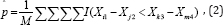
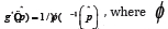
whereM=n₁ n₂ n₃ n₄, and the indicator function I(X_il - X_j2 < X_k3 - X_m4) = 1 if X_i1 - X_j2 < X_k3 - X_m4, otherwise I(X_fl - X_J2 < X_i3 - X_m4) =1. The De Neve and Thas [1] method for making inferences about p is based in part on a link function g (p) that maps the unit interval onto the real line. De Neve and Thas mention two possibilities: g(x) = x/(l-x) and the profit link function g(x) = ö^-1(x), where Ö(x) is the standard normal distribution. Let

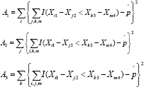
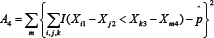
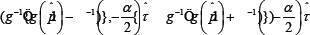
and

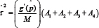
has a standard normal distribution. An approximate 1-α confidence interval for p is

This will be called method NT henceforth.

The basic percentile bootstrap method considered by Wilcox[4] is applied as follows. First, generate a bootstrap sample from the j^th group by sampling with replacement n_j observations from X_ij (i = 1, - - -, n_j ). Based on these bootstrap samples, estimate pusing(2) and label the result . Repeat this process Btimes yielding ( b = 1,---,B). B = 500 is used here, which seems to suffice in many situations in terms of controlling the probability of a Type I error[3]. However, a larger choice for B might result in higher power[5]. Put the in ascending order yielding . Let l=αB/2 and u= B - l . Then an approximate 1 - α confidence interval for P is . Let P* be the proportion of less than 0.5. Then form Liu and Singh [6], a p-value when testing (1) is2minmin(p* ,1-P*) . As indicated in section 3, NT can be unsatisfactory when the sample sizes are relatively small. Method PB performs reasonably well when the sample sizes are equal, but it can be rather unsatisfactory when the sample sizes are both relatively small and unequal. This suggests a simple modification. Let N = minmin{n₁,...,n₄}. Next, randomly sample, without replacement, N values from each of the four groups and let ^p be the resulting estimate ofp. Repeat this process L times yielding p. Here, L = 100 is used, which was found to generally give an estimate of p that is very similar to . Then inferences are made about p using the percentile bootstrap method previously described, except that bootstrap estimates of p are based on p^~rather than . This will be called method PB henceforth.

Simulations were used as a partial check on the small-sample properties of methods NT and PB. Simulation estimates of the actual Type I error probability, when testing at the 0.05 level, are based on 4000 replications. The sample sizes considered were (n₁, n₂, n₃, n₄) = (10,10,10,10) , (10,10,20,20), and (20,20,40,40). Data were generated from four types of distributions: normal, symmetric and heavy-tailed (roughly meaning that outliers tend to be common), asymmetric and relatively light-tailed, and asymmetric and relatively heavy-tailed. Specifically, data are generated from g-and-h distributions [7]. Let Z be a random variable having a standard normal distribution. If Z has a standard normal distribution, then by definition

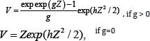
has a g-and-h distribution where g and h are parameters that determine the first four moments. The four distributions used here were the standard normal (g = h = 0), a symmetric heavy-tailed distribution (h = 0.2, g = 0.0), an asymmetric distribution with relatively light tails (h = 0.0, g = 0.2), and an asymmetric distribution with heavy tails (g = h = 0.2). Table 1 shows the skewness (ĸ₁) and kurtosis (ĸ₂) for each distribution. Hoaglin [7] summarizes additional properties of the g-and-h distributions. Once data were generated from one of these four distributions, (1) was tested using (σ_jX_ij) (i = 1,...,n_j;j = 1,...,4) . Three choices for the (σ₁, — ,σ₄) were used: (1,1,1,1), (4,4,1,1) and (1, 1,4,4). These three choices are labeled VP 1, VP 2 and VP 3. Simulations indicate that for VP 3, and when the sample sizes are unequal, both NT and PB perform reasonably well. That is, when the distributions with the larger variances are associated with the larger sample sizes, control over the Type I probability is fairly good. But for VP 2, this was no longer the case. So for brevity, only results for VP 1 and VP 2 are reported.

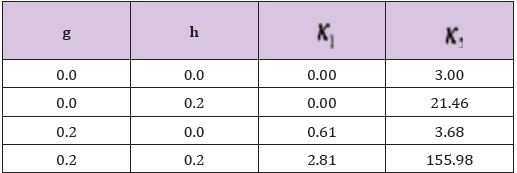
Table 1: Skewness (ĸ₁) and Kurtosis (ĸ₂) of the g-and-h distribution.

Table 2 summarizes the estimated Type I error probabilities. Although the importance of a Type I error probability depends on the situation, Bradley [8] suggests that as a general guide, when testing at the 0.05 level, the actual level should be between 0.025 and 0.075. Based on this criterion, method NT is unsatisfactory in nearly all of the situations considered. In contrast, method PB satisfies this criterion for all of the situations considered. Regarding method NT, it is noted that under normality and homoscedasticity, with n= (20,20,20,20),the estimated Type I error probability is 0.066. For n= (40,40,40,40) the estimate is 0.057. Also, simulation results reported by De Neve and Thas [1] indicate better control over the Type I error probability than indicated by Table 2 under normality, homoscedasticity and n= (10,10,10,10). It is unclear, however, which link function they used. Switching to the link function g (x ) = x /(l - x) , simulation estimates were more consistent with their results. That is, apparently, the choice for the link function is important. However, when dealing with unequal sample sizes and heteroscedasticity, estimated Type I error probabilities were consistent with those in Table 2. For example, for VP 2, g = 0.2 ,h = 0.0 and n= (10,10,20,20), the estimate was 0.09. Increasing the sample sizes to n= (30,50,70,90), again control over the Type I error probability is unsatisfactory. If instead all of the sample sizes are equal to 40, the estimate is 0.076, and for a common sample sizes of 50 the estimate is 0.067.

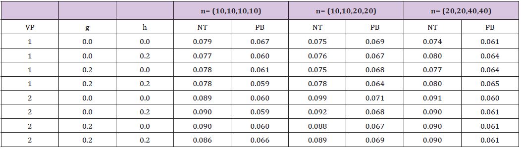
Table 2: Estimated Type I Error Probability, α=0.05.

Method PB is illustrated with data from the Well Elderly 2 study [9]. Generally, the Well Elderly 2 study was designed to assess the effectiveness of an intervention program aimed at improving the physical and emotional wellbeing of older adults. A portion of the study focused on measures of depressive symptoms. Here we compare measures for a control group to a group that received intervention while taking into account a second factor: participants who identified themselves as White, versus those who did not. First it is noted that when dealing with 20% trimmed means, a significant interaction is not found at the 0.05 level using the method in Wilcox[3] (section 7.4.1); the R function btrim was used. The p-value is 0.18. With no trimming, the p-value is 0.077. Comparing medians via a percentile bootstrap method (using the R function med2mcp), the p-value is 0.264. Using method PB, the p-value is 0.12. So, of course, the choice of method can make a practical difference. The suggestion is that by considering multiple notions of interactions, this provides a deeper and more nuanced understanding regarding the nature of the interaction. Even if say the 20% trimmed means had been significant, method PB provides a useful perspective: for randomly sampled participants from each of the four groups, there is an estimated 0.435 probability that the decrease in depressive symptoms, between the participants who describe themselves as White, is less than the decrease between participants who do not identify as White.

In summary, with equal sample sizes of at least 50, method NT performed fairly well. But otherwise, it can be unsatisfactory with respect to the Type I error probability. Of particular concern are situations where the sample sizes are unequal and there is heteroscedasticity. In contrast, method PB performed reasonably well in all of the situations considered, so it is recommended for general use. It is noted that method PB can be extended to testing linear contrasts when there are more than four groups [4]. The method used by Wilcox is based in part on a simple extension of , which was motivated by computational issues related to estimating the distribution of a linear combination of independent random variables. Here, this computational issue does not arise when using p^{^} unless the product of the sample sizes exceeds the capacity of the computer being used. As previously noted, a seemingly natural speculation is that ȕ is preferable to for the situation at hand, but the simulation results reported here indicate the opposite conclusion. Finally, the R functions WMW interci and inter WMWAP perform methods NT and PB, respectively. Both are being added to the R package WRS.

1. De Neve J and Thas O (2016) A Mann-Whitney type effect measure of interaction for factorial designs, Communications in Statistics - Theory and Methods.
2. Gao X and Alvo M (2005) A nonparametric test for interaction in twoway layouts. The Canadian Journal of Statistics 33(4): 529-543.
3. Wilcox R R (2017a) Introduction to Robust Estimation and Hypothesis Testing. 4^th (ed) San Diego, Academic Press, California, USA.
4. Wilcox R R (2017b) Linear Contrasts Based on an Extension of the Wilcoxon-Mann-Whitney Approach. International Journal of Statistics and Probability 6(3).
5. Racine J, MacKinnon J G (2007) Simulation-based tests than can use any number of simulations. Communications in Statistics Simulation and Computation 36(2): 357-365.
6. Liu R G, Singh K (1997) Notions of limiting p values based on data depth and bootstrap. Journal of the American Statistical Association 92: 266277.
7. Hoaglin D C (1985) Summarizing shape numerically: The g-and-h distribution. In D Hoaglin, F Mosteller, J Tukey (Ed) Exploring Data Tables Trends and Shapes. Wiley, New York, USA, pp. 461-511.
8. Bradley JV (1978) Robustness and Power of the Kornbrot Rank Difference, Signed Ranks, and Dependent Samples T-test. British Journal of Mathematical and Statistical Psychology 31: 144-152.
9. Clark F, Jackson J, Carlson M, Chou C P, Cherry B J, et al. (2012) Effectiveness of a lifestyle intervention in promoting the well-being of independently living older people: results of the Well Elderly 2 randomised controlled trial. J Epidemiol Community Health, 66(9): 782-790.