 Research Article
ABSTRACT
In this study, diagnostic nonparametric tests based on rank-sums of biomarkers and clinical variables were developed for predicting a binary response for organ failure dysfunction. The nonparametric approach is used in order to more effectively deal with the widely different dispersion scales of data within different biomarkers. It is shown that it performs better in terms of specificity and sensitivity statistics than other commonly employed methods such as sparse logistic regression, random forests and decision trees. A Bayesian posterior distribution and credible intervals on the probability of developing organ failure given that the diagnostic test is positive was then calculated, based on non-informative priors. Typical examples come from trauma data on biomarker and clinical variables from a first blood draw following critical injury, and we apply the developed methodology here to such a case. We conclude that the proposed nonparametric methods are well adapted to be applied to data with characteristics typically encountered in the trauma population.
Keywords and Phrases: Widely Dispersed Biomarker Data; Clinical Covariates; Multiple Organ Dysfunction; Nonparametric Inference
Introduction
Improvements in pre-hospital care and development of trauma systems lead outcomes following traumatic injury to expand from a focus on mortality to complications such as multiple organ dysfunction (MOD) and prolonged critical illness [1,2]. The overarching current clinical challenge is that of reducing shortand long-term morbidity through early-targeted interventions. We refer to (Lamparello, et al. [3]) for a detailed motivational narrative underlying the primary medical issues involved. A typical adverse outcome in such patients is Multiple Organ Dysfunction Syndrome (MODS) which peaks between 2 and 5 days after severe injury. It is, therefore, helpful to develop a method that predicts the occurrence of MODS early after arrival to a trauma center. To accomplish this, we used readings of inflammation biomarker levels and routine clinical variables obtained after arrival to our trauma center. From these readings, we sought to estimate whether there will or will not be the onset of organ dysfunction by five days post injury using an optimized MODS metric based on the Marshall MODS score [4], calculated on days 2 through 5 and defined as the average Marshall MODS score of days 2 through 5 (a MODS D2-D5). In addition, knowing the prevalence of developing organ failure from the available data, along with the sensitivity and specificity of our diagnostic test, we can compute the probability of a patient to develop MODS given that the patient has a positive test with our diagnostic. Our rank sum diagnostic test yields a sensitivity of 86% and specificity of 70% for predicting a MODS D2-D5 threshold. Other commonly used methods for such data, specifically sparse logistic, random forests and decision trees, yield sensitivity in the mid-sixties to mid-seventies and specificity in the mid-fifties to mid-sixties (using distance to point (0,1) on the Receiver Operating Characteristic (ROC) curve). In summary, we develop a tractable Precision Medicine scheme through a nonparametric rank based statistical method that helps in the early identification of trauma patients with high risk of developing elevated MODS scores by day 5 of ICU stay, allowing for a prognosticating tool that is likely to aid in clinical trial design and in patient care decision support.
Development of Nonparametric Models
Circulating inflammation biomarker data that are obtained from trauma patients involve rather different scales of measurement for each biomarker. For certain biomarkers there are occasional readings that are many times the median value; in one biomarker, for example, the maximum reading was over 1200 times the median value. These readings are not outliers, as they are found consistently. Such sweeping ranges in some biomarkers but not in all of them, make classification based on parametric analysis particularly challenging. We endeavored to standardize these biomarker responses as we sought classifiers that would allow good separation of patients with low MODS scores from those with high MODS scores. Among the standard techniques we applied were Sparse Logistic Regression, Random Forests, and Decision Trees. We then developed our own nonparametric rank-sum classification model that is described in detail below. A comparison of these four methods was obtained by training each model on the same 70% on the data and computing its performance on the remaining 30%; the performance is described in terms of sensitivity and specificity - the point on the ROC curve that is closest to (0,1). This was repeated 20 times. Table 1 summarizes the results. For this data set, and we believe for similar biomarker data, nonparametric models may prove to be better classifiers. Nonparametric techniques on biomarker data have been used in cancer treatment [5,6]. Further mention and ad hoc uses of nonparametric techniques applied to biomarker data are also found in Baker [7] and Shahjaman, et al. [8]. The nonparametric rank-sum method developed here may be viewed as a sparse all-regressions choice that either includes or excludes sets of variables; in this sense, it can also be interpreted as a Lasso model. We selected a percentage of data on which to develop and train our model and used the remaining data to predict the binary response. Initially, we converted the data to ranks. By restricting to main effects only, we sought the variables that yield the highest main effects with the response. This reduces the dimensionality of the data sufficiently so as to allow us to run all subsets of the remaining variables (as ranksum models) and monitor which variables occur most frequently. We found that often the best subset involves s variables, where s is typically approximately half the total number of variables from which we chose. With the best s variables identified, we proceeded in summing the ranks and use that as a nonparametric predictor of the binary response. The model selected was that which yields the pair (se, sp), of sensitivity and specificity, with both se and sp as high as possible. Realizing that these are dependent quantities controlled by the Receiver Operating Characteristic (ROC) curve, we selected (se, sp) such that (1 − sp, se) is the point closest to (0, 1) on the ROC curve.
Next, we sought to utilize the above model as a diagnostic tool having as input the biomarker and clinical variable data obtained from the first blood draw and as output either 1 (positive, or high MODS defined as a MODS D2-D5 > 3) or 0 (negative, or low MODS defined as a MODS D2-D5 < 3). This was used as a Bayesian setup for estimating the posterior probability of developing high MODS given that the diagnostic tool yielded a positive result. We based this on Binomial and non-informative Beta priors on the parameters to be estimated and simulated from the posterior Beta distribution to generate credible intervals for our estimates. The work in producing Table 1, as well as these rank-sum models, were developed using R (The R Project for Statistical Computing) and S-PLUS (Insightful Corporation. Seattle, WA). More specifically, we had 355 patients included in the construction of the model. The outcome used for identification of the prognostic variables was the average of MODS score measured daily on post-injury days 2 through 5 (a MODS D2-D5). An a MODS D2-D5 score ≥ 3 was defined as high MODS (recorded as a 1) and an a MODS D2-D5 score < 3 was defined as low MODS (recorded as a 0), in line with the clinical understanding on the onset of MODS. Our modeling process was as follows. In general, we denote by Y the binary response and by X1, X2, . . . , Xm the variables we used as potential predictors of Y . If the data on these variables were available on n subjects, we can view the data as a n × m matrix X (each subject corresponding to a row) with the ith column indexed by the variable Xi. Data on Y is a n × 1 vector having 0 and 1 as entries, with rows indexed by subjects in the same order as the rows of X. Next, we randomly, and without repetition, selected a “training Subset” of subjects (or rows of X) on which we built the model. We then used the remaining rows as a” testing-set” for the model we developed. In this trauma patient stratification application, we trained the model on 70% of the 355 subjects and tested it on the remaining 30%, where Xt and Yt denote the data matrix and response associated with the training set.
Selection of Significant Variables in the Training Set
We performed a screening for main effects of the columns of Xt by using Wilcoxon rank-sum tests for each column with the binary response Yt; then, we selected the columns that had significant p-values less than a fixed threshold. This often yielded reasonable variable choices, but we also utilized the following more robust approach, which casts a wider net for capturing significant variables by examining subsets of the “training set”. First, we fixed r, a number of rows of Xt. We then simulated s times (e.g., s = 10, 000) matrices with r rows randomly selected from those of Xt. For each choice, we performed a Wilcoxon rank-sum test to compute the vector of p values for each of the m variables with the correspondingly trimmed sub vector with r entries of Yt. Next, we averaged these s vectors of p-values. We next selected as significant variables those with average p-values less than a specified threshold. We suggest choice of r of 80% or more of the numbers of rows in Xt. This approach often yields significant variables that will differ from those obtained by merely restricting to the original columns of Xt. We also remark that while averaging of vectors of p-values can be done for a fixed value of s, incorrect inferences will result if such averaging is done for differing values of s. However, different values of s can be tried, and one can examine how consistent the average vectors of p-values are. In our particular application, this approach yielded a total of 14 variables with significant main effects, out of the initial 7 clinical and 31 biomarker variables available, using a p-value threshold of α = 0.03. Specifically, the variables were chloride (Cl), carbon dioxide (CO2), creatinine, partial thromboplastin time (PTT), platelets, IL-21, IL-23, IL-6, IFN-γ, IL-7, IL-8, IL-17A, IL- 10, and MCP-1. The matrix Xt for our data now consisted of these 14 columns. While restricting to main effects in our selection of variables hides possibly more subtle multifactor interactions, such dependencies are generally very difficult to model successfully in biological responses which, unlike engineering uses, are typically difficult to replicate.
Further Variable Reduction and Interpretability
Whenever possible, we aimed to produce models that are intuitive and as simple as possible, subject to providing a reasonable explanation of the existing data and the underlying biological phenomena. With this at heart, we used ranks (rather than raw data); this immediately goes a long way in addressing issues of occasional large swings in certain biomarker readings. Ranks also, by their very nature, normalize the variables and rank-sum models extract just subsets of significant variables, rather than weighted sums. We thus restricted to rank-sum models. Among columns of Xt (all with p-value < α), some have positive and others negative Wilcoxon rank statistics. We therefore replaced each column with a negative Wilcoxon statistic in Xt by its negative in order to associate high ranks only with large positive values. This simplified the rejection region for a rank test. We next denoted by Rt the matrix obtained from Xt by replacing (so modified) entries in each column by the corresponding ranks. Through the process of dimensionality reduction, we reduced the number of columns of Xt from m to k (≤ m). Hence, Rt has k columns.
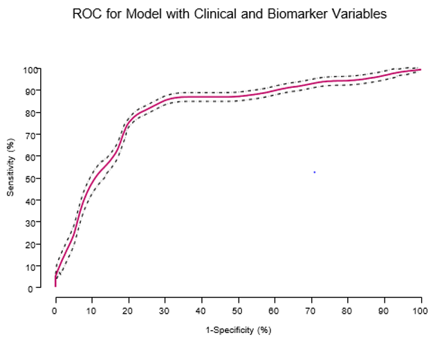
Figure 1: Receiver operating characteristic (ROC) curve for the prognostic model derived using data from the derivation cohort. ROC curve for the model based on the combination of admission clinical variables and inflammation biomarkers (sensitivity = 86% and specificity = 70%), AUC = 0.78 (out of 1.0).
For values of k within a manageable computational range (typically less than 30), we examined models of the following form. First, we selected a subset of s columns of Rt and summed them up to obtain vector Vs. We considered Vs a possible model to predict Yt. Specifically, we decided that the entries in Vs that are ≥ a cutoff c predict a 1 in Yt; the rest predict 0. Cutoff c was chosen so as to optimize the vector (sensitivity [se] and specificity [sp]). If this approach seemed too exhaustive (not being a linear order), we optimized the sum of se and sp. Typically, we wanted both entries se and sp to be as large as possible. The approach is similar to” all-regressions” in the more common non-discrete parametric settings. Working on the” training set”, the best model that emerged comprised the following variables: CO2, creatinine, PTT, IL-6, IL-7, IL-10, and MCP-1. We note that the biomarker variable IL-7 was negated, that is, its sign was changed in Xt. The performance of this model in the” testing-set” yielded (se, sp) = (0.86, 0.70), the closest point to (0, 1) on the ROC curve. The ROC curve for the model appears in Figure 1, with an area under the curve (AUC) of 0.78 (out of 1.0).
Bayesian Inference on the Probability of Developing Mods (Table 1)
In the previous sections we constructed a rank-based diagnostic
test that predicts the onset of MODS from biomarkers and clinical
readings obtained from the earliest blood draw upon admission
to the ER. The sensitivity and specificity rates for this diagnostic
test were 0.86 and 0.70, respectively. Also known, from the data
and possibly medical literature, is the prevalence rate of MODS in
critically injured patients - it is 68/355 = 0.192, or about 1 in 5 in
our data. Of interest is the estimation of the probability p that a
critically injured patient develops MODS knowing that the patient
tested positive by our diagnostic test. We use known techniques,
found in Berger [9], to formulate an answer. Denote by p0 the
(unknown) prevalence rate of MODS for the population of critically
injured patients; our best estimate for p0 is pˆ0 = 0.192 that we
mentioned above. The theoretical sensitivity rate of our diagnostic
test is not known and denoted by p1; our estimate from data is
 . Likewise, for the specificity rate we have 1-p2 estimated
from our diagnostic test as
. Likewise, for the specificity rate we have 1-p2 estimated
from our diagnostic test as  . If p denotes the
theoretical probability that a patient that tested positive by our
rank-based diagnostic actually has MODS, then an application of
Bayes rule immediately yields:
. If p denotes the
theoretical probability that a patient that tested positive by our
rank-based diagnostic actually has MODS, then an application of
Bayes rule immediately yields:
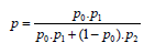
Substituting in our estimates immediately yields a point
estimate for p; it is  . In summary, knowing that a patient
tested positive on our rank based diagnostic test more than doubles
the patients’ chances of developing MODS by day 5 in the ICU.
. In summary, knowing that a patient
tested positive on our rank based diagnostic test more than doubles
the patients’ chances of developing MODS by day 5 in the ICU.
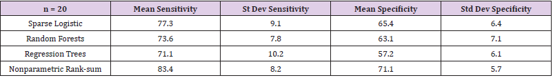
Table 1: Twenty simulations from our data show the mean and standard deviation of the sensitivity and specificity values obtained for each of the four methods used. The models were obtained by using a training set of 70% and testing set of 30% from our data set.
Constructing Credible Intervals
With p0 , p1 , p2 as defined above, in our data we estimate
pi by  ,. Here n0 is the number of patients in our data,
and x0 is the number of patients in the data that have MODS;
consequently,
,. Here n0 is the number of patients in our data,
and x0 is the number of patients in the data that have MODS;
consequently,  is the estimate from our data of the
prevalence of MODS in the population of traumatically injured
patients at large. By n1 we denote the number of patients in our
data known to have MODS who underwent the blood test, and x1
is the number of such patients on which the test was positive; thus
is the estimate from our data of the
prevalence of MODS in the population of traumatically injured
patients at large. By n1 we denote the number of patients in our
data known to have MODS who underwent the blood test, and x1
is the number of such patients on which the test was positive; thus  (estimate of sensitivity). Likewise, 2 n
is the number of patients in our data that do not have MODS but tested positive; in our case
(estimate of sensitivity). Likewise, 2 n
is the number of patients in our data that do not have MODS but tested positive; in our case  is equal to 1
− specificity.
Assume that the i x written above are realizations from the
Binomial ( ηi , pi ) distribution i = 0,1,2 . We place the uninformative
is equal to 1
− specificity.
Assume that the i x written above are realizations from the
Binomial ( ηi , pi ) distribution i = 0,1,2 . We place the uninformative  also known as the Jeffries prior - as prior distribution
on , pi, i = 0,1, 2. Then the posterior distribution for pi , after the
data i x is observed, has probability density function proportional
toU , which is the
also known as the Jeffries prior - as prior distribution
on , pi, i = 0,1, 2. Then the posterior distribution for pi , after the
data i x is observed, has probability density function proportional
toU , which is the  distribution. We can
now generate credible intervals for p by simulating out of
these Beta distributions. Randomly pick an observation pi
from each of
distribution. We can
now generate credible intervals for p by simulating out of
these Beta distributions. Randomly pick an observation pi
from each of  . Register the value
  Repeat this process 5,000 times. Determine
numbers L and U such that of the 5,000 values generated
Repeat this process 5,000 times. Determine
numbers L and U such that of the 5,000 values generated  percent are lower than L and percent are greater than
U. The interval (L, U) is a 100α% credible interval for the unknown
parameter p . Recall that the point estimate for p is 0.4. With our
data we performed such a simulation, by writing a quick program in
R, and obtained the following 90% and 95% credible intervals for p,
respectively: (0.314, 0.497) and (0.302, 0.514).
percent are lower than L and percent are greater than
U. The interval (L, U) is a 100α% credible interval for the unknown
parameter p . Recall that the point estimate for p is 0.4. With our
data we performed such a simulation, by writing a quick program in
R, and obtained the following 90% and 95% credible intervals for p,
respectively: (0.314, 0.497) and (0.302, 0.514).
Acknowledgement
This work was supported in part by the National Institute of Health, grant P50-GM- 53789.
References
- Glance LG, Osler TM, Mukamel DB, Dick AW (2012) Outcomes of adult trauma patients admitted to trauma centers in Pennsylvania, 2000-2009. Arch Surg 147(8): 732-737.
- Xiao W, Mindrinos MN, Seok J, Cuschieri J, Cuenca AG, et al. (2011) Inflammation, Host Response to Injury Large-Scale Collaborative Research, P. A genomic storm in critically injured humans. J Exp Med 208(13): 2581-2590.
- Lamparello AJ, Namas RA, Constantine G, McKinley TO, Elster E, et al. (2019) A conceptual time window-based model for the early stratification of trauma patients. J Intern Med.
- Marshall JC, Cook DJ, Christou NV, Bernard GR, Sprung CL, et al. (1995) Multiple organ dysfunction score: a reliable descriptor of a complex clinical outcome. Crit Care Med 23(10): 1638-1652.
- Graziani R, Guindani M, Thall P (2015) Bayesian nonparametric estimation of targeted agent effects on biomarker change to predict clinical outcome. Biometrics 71(1): 188-197.
- Kozak K, Amneus MW, Pusey SM, Su F, Luong MN, et al. (2003) Identification of biomarkers for ovarian cancer using strong anion-exchange ProteinChips: Potential use in diagnosis and prognosis. PNAS 100(21): 12343-12348.
- Baker SG (2000) Identifying combinations of cancer markers for further study as triggers of early intervention. Biometrics 56(4): 1082-1087.
- Shahjaman M, Rahman MR, Islam SMS, Mollah NH (2019) A Robust Approach for Identification of Cancer Biomarkers and Candidate Drugs. Medicina 55(6): 269.
- Berger J (1985) Statistical Decision Theory and Bayesian Analysis (2nd)., New York: Springer Series in Statistics.
