 Research Article
Abstract
Economic vitality is an important indicator of economic development. In this paper, we have created a panel data model to analyze the influencing factors of economic vitality in China. We conducted the following studies. Using the correlation analysis, the correlation among various elements is revealed to be strong, which denies the independence null hypothesis. By establishing VAR-VEC model, the long-term and short-term effects of economic policies on economic vitality in Beijing are analyzed. It is showing that the population changes and enterprise vitality have a positive impact on economic vitality with the influencing factors being 0.01 and 0.07, respectively. At least three cointegration relationships between time series exit using the ADF unit root test and Johansen cointegration test. We use Ais-Sc Criterion to determine the order of delay as the third order and OLS estimation method to get the coefficients of VEC Model. Because of experience accumulation, the economic vitality follows a W-shaped trend. Utilizing the minimum average deviation method to preprocess the index data, 9 representative indexes are obtained. We then extract two main factors by factor analysis and build an index system of economic vitality. The economic vitality of each city from 2009 to 2020 is calculated based on this index system. Beijing, Shanghai, Guangzhou and Shenzhen often rank first, while Kunming and Dongguan often rank last. The panel data model test results are like that of index system on the same data. Finally, the previous conclusions have been reviewed. The ORT development strategy to improve economic vitality is advised.
Keywords: Panel data model; VAR-VEC model; Factor analysis; Index system
Introduction
Under the background of the new age, China’s economic, social, cultural, ecological, political and other fields are coruscating new vigor and vitality. At the same time the good life is people’s increasing need to inadequate and unbalanced of the contradiction between the development of becoming the social contradiction, and the unbalanced economic growth between different regions is the concentrated reflection of unbalanced is not fully developed; To accelerate the narrowing of the gap in local economic growth, promote the vigor of regional economic growth, and promote the coordinated growth of a regional economy is the basis and key to solving the main social contradictions in the new age, and is also the driving force of economic and social development axis. Regional economic vigor is a part of comprehensive local competitiveness. In recent years, to improve economic vitality, some regions have introduced a lot of preferential policies to stimulate economic power, such as reducing the approval steps for investment, providing financial support for entrepreneurship, and lowering the threshold for settling down to attract talents. However, due to distinct resource endowments, these policies have distinct affects in distinct regions. How to grasp the key factors and effectively improve it is a worthy research topic.
To study how to improve the regional economic vitality, this paper takes some cities in China as an example, selects several indicators to measure it, constructs the index system, and studies the relationship model of the influencing factors of it and considers the influence of population change trend and enterprise vitality change on the regional economic vigor change. At the same time, it analyzes the short-term and long-term impact of economic policy transformation on the economic vitality of various regions. At present, scholars at home and abroad rarely make more research on economic vitality, so this paper hopes to establish a mathematical model to analyze and measure regional economic vitality, and sort the economic vitality of some cities, to better extend the economic vitality analysis model to more research fields.
Models
Panel Data Model
Based on the panel data model, it collects data from various provinces and cities, performs correlation test and principal component analysis on the data. The fixed effect test and random effect test was carried out for the obtained factors. And the influence of policy and enterprise vitality on economic vigor was dissected based on the established relationship the model between each element and economic vigor.
Data Analysis and Processing: Based on the collected data has error and deficiencies, to reduce the invalid, the influence of the error data of the following model, improve the reliability of data, need to collect the data pretreatment, firstly the filtered data, remove abnormal data, secondly, proper supplement of incomplete data, finally, has correlation data linear regression analysis forecasting and slight fluctuation data using the moving average method to fill the missing value, to further improve the accuracy and the integrity of the data.
a) Data Selection Principle: This paper needs to collect alien indicator data describing economic vitality and influencing economic vigor, and the following classical indicators can be obtained according to the expert method and the literature [10,11,13,14]. Dependent variable. In the existing economic vitality research and analysis, more choose gross domestic product (GDP) as a measure of it. In this paper, to measure regional economic power, main elements from the effects of the economic vigor that reflects the GDP growth rate as the level of economic development during the period of change degree of dynamic indexes, namely whether a national economic basic index of the moving and USES the linear regression analysis and panel data model analysis, the main measures for regional economic vitality.
Independent variables. Based on the existing literature research outcomes and the above analysis, this paper selects nine aspects. It includes population growth rate, fiscal expenditure, and employment rate (mainly used to reflect the main influencing factors of local economic vitality and its growth trend). The employment rate is expressed by the number of unemployed; At the same time, in the establishment of the model, for the negative value of population growth rate, to reduce the error in the large number region. Dummy variables can be used instead of the original statistical samples, which are reset to zero in this paper. Control variables. Based on the analysis of the comprehensive evaluation index system of urban economy. Considering the availability of data, this paper introduces independent innovation ability, per capita length of education, professional and technical talent inflow and other irrelevant variables as control variables. Through analysis, the variables other than independent variables that can affect the change of dependent variables should be well controlled and regarded as constants to obtain appropriate causal relationship and attain the accurate value Table 1.
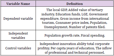
Table 1.Variable definition.
b) Independence Test: In the analysis of the relationship between the factors affecting economic vitality, to fully understand whether there is an internal relationship between the elements. According to the processed data, this paper carries out an independence test for each element. The data source is the national bureau of statistics, and the independence test is executed on the pre-processed data. See the appendix for the specific data. Make the following assumptions about the research hypothesis:
a. Null Hypothesis: The factors that influence positive energy are independent of each other.
b. Alternative Hypothesis: The factors influencing economic vitality are not independent.
Firstly, a chi-square independence test was executed. SPSS was used to conduct independent test for each influencing element to observe whether there was any correlation between each factor. The test results are as follows: It can be seen from Table 2 that the cross relation between each factor and the year. The cross table shows the availability of different influencing elements which occupies a complete percentage. It indicates that the opted data are valid values with high accuracy, which can be further compared in pairs to test the independence of judgment elements. The significance analysis is used to determine whether there is independence between factors. The chi-square significance test results are shown in Table 3. It can be seen from Table 3 that the degree of freedom is the probability of Person chi-square, which is less than 0.05. And the null hypothesis is rejected. The influencing factors are not independent of each other.
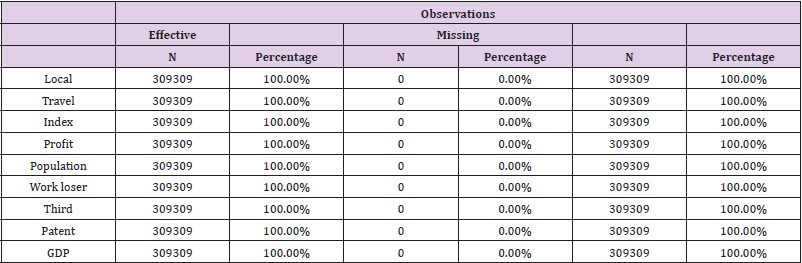
Table 2.Independence test results.
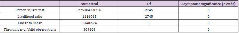
Table 3.Chi-square significance test results.
c) Correlation Analysis: Each factor in the collection is the indicator data of each city in the country, which belongs to the panel data. There may be a correlation between the data. Considering the correlation among various elements, the linear strength relationship diagram of each element is attained based on the data as follows: As can be seen from the observation in Figure 1, there is a correlation among all factors, and the expression form and strength of the relationship among all elements. The closer the data is to 1, the stronger the correlation is. Local GDP is positively correlated with Government expenditure Gross income from international tourism Consumer price index Education funds Total corporate profits Population Unemployment and added value of the tertiary industry, and negatively correlated with the number of patent applications. SPSS was used to conduct a correlation analysis on the data and the outcomes were shown in Table 4.
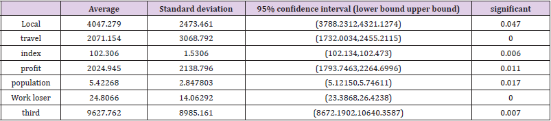
Table 4.Correlation analysis.
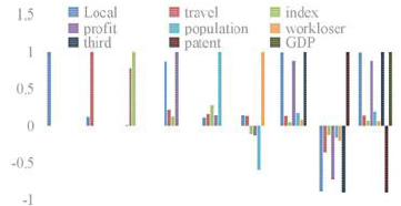
Figure 1: The linear strength relationship between the factors.
Correlation coefficients can quantitatively describe the closeness of linear relationships among elements. And SPSS is used for correlation analysis to attain the correlation coefficients among the influencing factors, as shown in Table 5. According to the above correlation analysis Table 5, there is a correlation among all factors. And the positive correlation coefficient is distributed between 0.5 and 1 reflecting a strong correlation. According to the significance test of the correlation coefficient, the significance values are all less than 0.05. It indicates that the correlation coefficient has reached a high level of significance. Therefore, there is a strong correlation between various elements are influencing economic vitality.
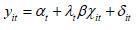
Establishment of Model: This section is based on the panel data of various factors collected from 31 provinces and cities in China from 2009 to 2020. Considering the influence of multiple factors on economic vitality, various methods can be used, such as multiple linear regression and panel data model. Here, a rough comparison is made before further model establishment. Compare the panel data model with the multiple linear regression model, as shown in Table 6. Based on the data and problem in this question, the panel data model is a better choice. The panel data model includes both the cross-section and the time dimension. Here, the elements affecting economic vigor are taken as the cross-section. And the year is taken as the time dimension. Where, i (i=1…8) represents the following linear model set for the year:
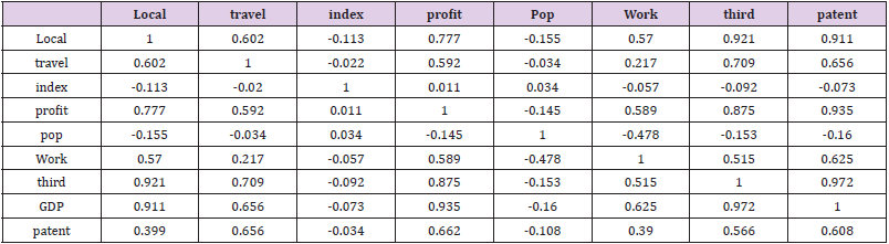
Table 5.Correlation coefficient result.
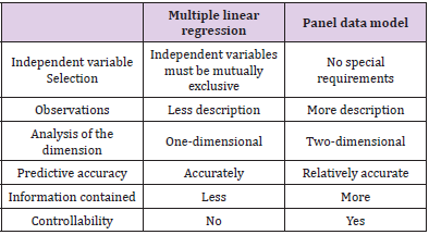
Table 6.Model comparison.
The panel data model can be further divided into fixed effect model and random effect model.
a. Fixed Effect Model
The individual affect is regarded as a stable factor that does not change with time, then equation one can be expressed as a vector.
In the formula, AT is a column direction where all elements are 1, and the others have the same meaning as the original model.
b. Random Effect Model
The individual affect ai is regarded as a random factor that changes with time. By using the random effect model, the long-term elements and short-term elements in the variance can be separated. The setting of the model is as follows:
c. Model Determination Based on Hausman Test
Because the missing related variables are not excluded, there will be dependent. Variable- local GDP will change with the same period correlation of random interference items. And the constraint conditions of exogenous variables are not satisfied so that the OLS estimator is biased and different. OLS is used to test the fixed-effect model. And GLS is used to test the random effect model. According to the reference [13], the difference between the random effect model and the fixed effect model is that it is difficult to try to make a high degree of distinction on the description of individuals. The stable affect will cost more degrees of freedom, while the random affect is more universal. The proposed the Hausman test can be used to distinguish them to some extent (Figure 2). Advanced random effect model test, test results are stored; Then the stable effect test is carried out on the model and the outcomes are saved at the same time. Finally, the Hausman test is performed on the outcome to obtain the final model. The method to verify that both models are satisfied is established in turn.

Figure 2: Inspection process.
It can be seen from the output that the parameter estimation variance of random and fixed- effect models under this test is a positive definite matrix, which satisfies the test conditions. Under the 95% confidence interval, the P-value is much less than 0.05. Therefore, the fixed- effect model should be opted as the explanation model for the influence of economic vitality, while the random effect model should be opted instead.
Model solving Process: In this section, stability analysis is conducted on the existing panel data, fixed-effect test and random effect test are executed on the whole data based on the panel mathematical model, and Hausman test is used to define the applicable model for the panel data. Finally, the analysis outcomes are attained based on the panel regression model.
A. Data stability and reliability analysis: The data of this paper comes from China National Statistical Yearbook, which includes the local government’s financial expenditure, the total income of local international tourism, consumer price index, total profits of enterprises, population, unemployment, tertiary industry, total patents, and local GDP. The inconsistency of the order of magnitude of each part will cause trouble to the model fitting. According to the statistical yearbook, the city is divided into 1-31. The distribution of various data is shown in Figure 3. Take Figure 3 for example, standardize it first. Assume that the original data is xm, after standardization is Xm, and Xni
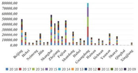
Figure 3: Data distribution of influencing factors in each city.
After attaining standardized data, it is shown as follows. It can be seen from the observation Figure 4 that after the standardization, the feature expression is clearer, which is conducive to the next model inspection work.
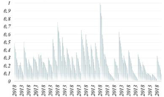
Figure 4: Standardized data distribution.
B. Fixed Effect Test Based on OLS: Panel data has the characteristics of separating long-term variables and short-term variables, while the fixed-effect model focuses on the relationship between variables within the group, it is necessary to test the fixed effect model. The estimation method is OLS estimation, two assumptions of the fixed-effect model are made.
Hypothesis 1: 
Hypothesis 2: 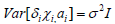
Theξ in Hypothesis one is the independent variable interference term.
Hypothesis 1: Assume that the does not affect the observed value, unobserved value, and post observed value.
Hypothesis 2: The general test of homogeneity. Ensure that the model satisfies the blue estimate of OLS. And organize data into long data types.
The year (2009-2020) is the cross-section marker, the province (1-31) is the research individual. And each type of independent variable is the influencing factor. The solution is based on Stata software, and the outcomes are shown in Table 7. Among them, the F value is very close to 0, indicating that the fixed effect is very significant in this case. Among the seven independent variables, the consumer index and unemployment rate are not significant within the 95% confidence interval. Local government expenditure, total tourism income, total profits of enterprises, resident population, and tertiary industry income have statistical significance. The statistics are shown in Table 8. Among them, the third industry has the most significant impact on GDP, and the consumer the index has the least influences on GDP. We can know that all the opted indicators have positive significance for GDP growth within the statistical range. It shows that this test has adopted hypothesis one and hypothesis two for panel data. And both are true.
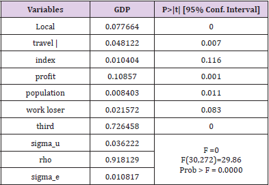
Table 7.Fixed effect test model.
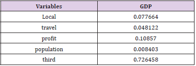
Table 8.Indicators passing the fixed effect test.
C. Random Effect Model Test Based on GLS Estimation
The number of indexes (N) is 10 and the period (T) is ten years.
In this case, it is also possible to meet the random effect model; the further test of the random effect model is needed.
Hypothesis 1: 
Hypothesis 2: 
Hypothesis 3: 
Hypothesis 4: 
Hypothesis 5: 
According to the above assumption, suppose that the distribution of each independent variable is constrained in a specific case. And the effect of each independent variable obeys the mean value of 0. The second is the description of random interference, which is not correlated with explanatory variables. The third term makes the two coefficients independent of each other. Based on the above description, the GLS estimation method can be used to obtain whether the panel data model conforms to the random effect test when the collected variables are close to the period. Organize data into long data types. The year (2009-2020) was used as the cross-section marker, the province (1-31) as the study individual, and each type of independent variable as the influencing factor. Use Stata software to solve the problem and get the outcomes, as shown in Table 9.
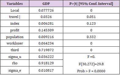
Table 9.Test results of random effect mode.
In 95% confidence interval, P value is 0 five hypotheses are passed in this case. This case is suitable for the random effect model (Table 10). The third industry has the most significant impact on GDP, and the resident population has the least influence on GDP. We can know that all the selected indicators have positive significance for GDP growth within the statistical range. At the same time, it shows that the test has passed all the hypotheses of panel data and satisfies the random effect (Figure 5). The number of indexes (N) selected in this paper is 10 and the time span (T) is 10 years. In this case, both the fixed effect model and the random effect model are satisfied, and the further model test is needed. At this time, the Hausman test should be taken.
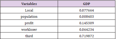
Table 10.Indicators passing the random effect test.

Figure 5: When both tests pass.
D. Model Determination Based on Hausman Test: According to the reference [13], the difference between the random effect model and the fixed effect model is that it is very difficult to distinguish them to a high degree in the description of individuals. The stable effect will consume a large degree of freedom. At meanwhile, the random affect is more universal on this basis. The proposed Hausman test can be used to distinguish them to some extent. The test of the advanced random effect model will store the test results, then test the fixed effect of the model and save the outcome. The Hausman test is used to get the final model. Then the method to test the two models simultaneously is built (Table 11). It is known from the output that the variance of parameter estimation of random and fixed effect models under this test is a positive definite matrix, which satisfies the test conditions. Under 95% confidence interval, P-value is far less than 0.05. Therefore, we should choose the fixed- effect model as the explanation model of economic vitality.

Table 11.Hausman test results.
E. Analysis of Model Test Results: Using the Hausman test, the fixed-effect model is determined as the interpretation model of economic vigor, and the outcomes are shown in Table 12. Among them, the factors that have a positive influence on economic vitality (GDP) are the local government financial expenditure, the total annual revenue of local tourism, the total annual profit of local enterprises, the local permanent population, and the GDP of the tertiary industry. According to Figure 6, based on the fixed-effect model, it can be concluded that the tertiary industry has the largest influence on the estimated vitality. It followed by the annual income of enterprises (enterprise vigor), the input expenditure of local government (policy bias), the total income of local tourism, and finally the permanent population. Among them, the influence of the tertiary industry on economic vigor is more than seven times that of enterprises. It indicates that the third vigor can occupy most of the effect among the factors influencing it.
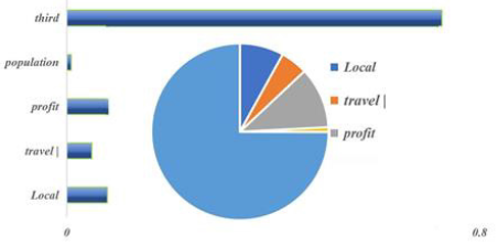
Figure 6: Contribution degree.
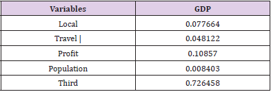
Table 12.Test results of the fixed-effect model.
F. Activation Scheme Proposed Based on the Fixed- Effect Model: According to the fixed-effect model shown in Figure 4, the explanation degree of each factor to economic vitality has been given. And the following Suggestions are given according to the influence degree.
i. To increase the proportion of the tertiary industry in the overall economy, the tertiary industry plays an important role in the influencing factors. So, it is necessary to strengthen the overall proportion of the tertiary industry in the current stage of social construction. Raising the economic proportion of the tertiary industry will promote the improvement of economic vitality.
ii. In the process of development, the region should combine its resource endowment and industrial foundation to find the optimal ratio of enterprise structure. And it will complete the adjustment of enterprise structure as soon as possible and develop appropriate leading industries to promote economic growth. It will be conducive to a steady increase in economic vitality.
iii. Local government expenditure has an impact on economic vitality. The government needs to be tightly managed to make its spending transparent. We will increase government support for enterprises.
iv. Entrepreneurship is encouraged. The government takes the lead in encouraging entrepreneurship and social practices are carried out to transform enterprises.
According to the influence of individual factors on economic vitality attained from the fixed model, the influence law of elements is summarized, among which policy adjustment (government expenditure) and enterprise vigor (total annual profit of enterprises) have a positive influence on economic power, and the implementation of policies in this respect should also be intensified.
G. The Influence of Changing Trends of Population and Enterprise Vigor on Economic Vitality
Seven variables were opted, GDP was taken as the expression of economic vitality, and the fixed-effect model in the panel data model was used to draw the following conclusions: The growth rate of the permanent resident population has a positive impact on economic vitality. The increase of permanent resident population will increase economic vigor in a small extent. If the population grows too fast, it will increase the rate of job competition and lead to the rise of unemployment, which will hurt economic vitality. However, the growth decline of enterprise vigor directly affects economic power and presents a positive correlation change.
The Establishment of the VAR-VCE Dynamic Volatility Model
Based on the panel data, this section intercepts the local government expenditure of Beijing as a representation of economic policy and establishes a vector autoregressive model (VAR). Taking economic vitality as the research object, the stability of each factor is verified. Based on vector error correction model (VEC), the lag order and influence function response chart are given to describe the long-term and short-term influence of policy implementation on it.
Data Preparation: Based on the cross-section data of Beijing in the panel data of the whole country, this section conducts relevant test and Analysis on the data. Finally obtains five significant factors that have an influence on the economic vitality: local per capita GDP, local government expenditure, local tourism gross income, local people’s living consumption index, and local resident population. Among them, five kinds of data of Beijing, local per capita GDP, local government expenditure, local tourism gross income, local people’s living consumption index, and local resident population is given in Figure 7 after standardization. It can be seen from Figure 7 that the local government expenditure has an increase in each year, basically showing a linear growth. There is no significant change in the local tourism income, which is relatively stable compared with other indicators. It indicates that Beijing, as the capital of the country, is very successful in the construction of tourism culture. The resident population gradually declined after reaching the peak from 2012 to 2013, which indicates that Beijing’s population has changed largely, and its GDP has grown steadily. It is not obvious that GDP is affected by the fluctuation of alien factors. To understand the dynamic influence of various elements on GDP, we need to carry out vector autoregression for this group of data.
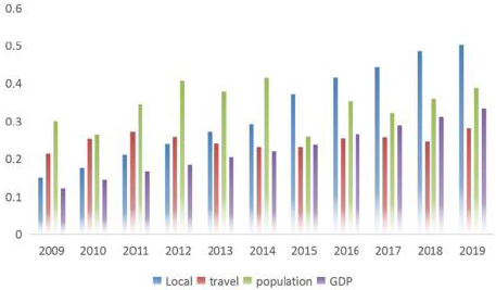
Figure 7: Normalized back view.
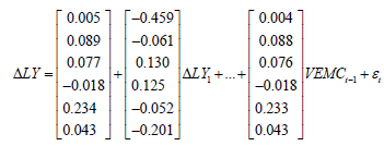
The Establishment of Vector Autoregression (VAR) Model: Based on the statistical properties, a function containing the lag value of exogenous and endogenous variables are established to construct the model, which illustrates the influence of the dynamic changes of variables on the dependent variables. VAR model is essentially a model of multi equation class. Based on the moving changes of multiple variables, the interaction between alien variables is investigated. Any endogenous variable in the equation system is constructed to express the lag term of any variable. Its general expression is

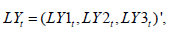
Where Yt is the endogenous variable vector of K dimension, Yt-i (i=1,2,…,p) is the vector of endogenous lag variable, Xt-i is the d-dimensional exogenous variable vector or lags exogenous vector. P and R are the lag orders of endogenous and exogenous variables, respectively. Ai is a k-order coefficient; Bi is a k-row-d-column coefficient matrix, these matrices need to be estimated by specific methods. The last term is a vector composed of k- dimension random error terms. According to the solution of the following figure, we can get the estimation coefficient (Figure 8). Firstly, the lag order of the AVR model is determined according to the AIC information criterion and SC criterion when the minimum value is taken. Then the lag order is substituted into the meta model, and the coefficient of the AVR model can be obtained by the OLS estimation.
The Establishment of the VEC: When multiple time series are unstable, the Johansen method is used to test whether there is a cointegration relationship. If there is co integration relationship, the VEC model can be established to analyze the dynamic relationship of its multi pass model.

Figure 8: Model inspection process.
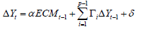
In the formula, ECMt-1 is the error correction term. Compared with the AVR model. The error correction term is an important feature to distinguish the two. The error correction term reflects the long-term equilibrium relationship of each variable, and the deviation of long-term equilibrium can be corrected by quick shortterm adjustment. Before building the VEC model, the Johansen test is needed to define the stability and reliability of the model.
Model Summary: To determine the regression type of a group of vectors, we need to conduct multiple tests. Finally, we can define whether the model has a correction term. Next, we summarize the model to construct a complete the VAR-VEC model.
Solution of the Model: In this section, we first judge the stability of time series and then do the ADF test on vector series to decide its stability. Then, the first order and second-order’s difference are used to judge its stability. The cointegration test of the original data is carried out. And the satisfied model type is attained. Finally, the stability of the model is judged. And the moving influence of policy implementation on economic vitality is obtained.
1) The ADF Unit Root Test of Vector Sequence: First, all the time data are tested by the ADF test, and the distinct order is 0. The lag order is 1-2, and the test results are shown in Table 13. It can be seen from Table 13 that under the time test of order 0 raw data, the t-values of six kinds of t-tests are greater than the comparison data under the confidence interval of 95%, shows that the time series of this group of data does not pass the ADF test of the original data, and the further differential test is needed. Carry out difference differentiation on the original data and continue the ADF test on the data after difference. And the outcomes are shown in Table 14. It can be seen from Table 14 that under the ADF time series test, the T value of population t test in six species is less than the comparison data under the confidence interval of 95%. Among the six kinds of data, only the population has passed the first-order difference test. The first-order difference of this group of data is not zero. So, a further difference test is needed.
Carry out the second-order difference differentiation on original data and continue the ADF test on the data after the difference and the outcomes are shown in Table 15. It can be seen from Table 15 that all the data after the second-order difference have passed the ADF test this group of data is zero in the second order, and then the inter group cointegration test is carried out. Figure 9 shows the visual information of three points of each variable under three tests. The confidence intervals of the middle three levels are 1%, 5%, and 10% respectively. After the first-order difference, the only population passed the test. After the second-order difference, all the data pass the test. And the group of data is the second-order zero integer data.
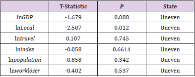
Table 13.zero-order difference ADF unit root test results.
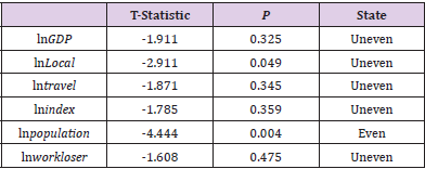
Table 14.ADF test results after first-order difference.
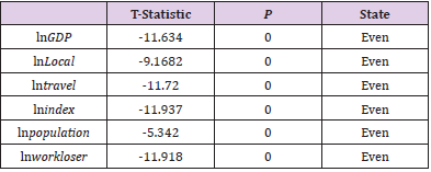
Table 15.ADF test results after first-order difference.
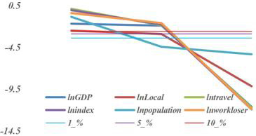
Figure 9: Visualization of three tests.
2) Johansen co Integration Test of Variables: According to the ADF test, the original variable is a second-order zero integer sequence; that is to say, the original variable is an unstable sequence. First, the Johansen co integration test is carried out to find out whether there is a co integration relationship between its combinations. The test method is to calculate the trace statistics trace and the maximum eigenvalue Max eige value. Using the cyclic statistical hypothesis, the existence of a cointegration logarithm is assumed. Table 16 shows the Johansen co integration test results. From the trace statistics trace in Table 16, it is assumed that none is the sequence without cointegration.
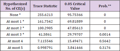
Table 16.Cointegration test results.
Under this assumption, the trajectory value is 255.6213, which is greater than the critical value of 95.7537. If the original hypothesis is rejected, there is at least one cointegration relationship. In the case of 5% confidence level, the original assumption is that there are at least four sets of cointegration relationship. Its trajectory value is less than the critical value. And the determination of the fourth set of cointegration relationship is rejected by the assumption. There are at least three cointegration relations in the linear combination of time series with surface instability.
Establishment and Solution of VEC Model: When the original data series are non-stationary time series and Johansen cointegration test shows that there are at least three cointegration relationships in the series. To build a proper VEC model, it is necessary to determine the optimal lag order of the model. The stability of the model is explained by the AR root graph and Roland causality analysis. Finally, the impulse response chart is given, and the long-term and short-term effects of policy implementation on economic vitality is dissected.
1) Determination of Lag Period Based on AIS-SC Minimization Criterion: When the model is not integrated and stable, multiple VAR models with different lag periods can be established first. According to the relationship of multiple research variables, the values of each AIC and SC can be recorded and compared. The optimal lag period of the model can be selected according to the theory of reaching the minimum simultaneously. The outcomes in Table 17 are calculated by Eviews software (Figure 10). It can be seen from Table 17 that the AIS value decreases with the increase of VAR (N) lag period, presenting a monotonic decreasing state. The SC has a minimum at VAR (3). According to the AIS information standard and SC standard, the optimal lag time is opted as the third-order lag time.
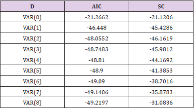
Table 17.AIS-SC calculation results.
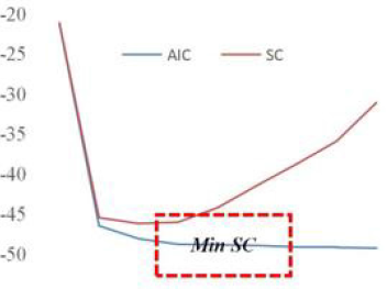
Figure 10: Model inspection process.
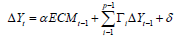
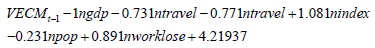
2) Determination of VEC Model Parameters: According to the above analysis, through the cointegration test, there are at least three groups of cointegration relationships between time series. It can be used to build the EVC model. According to the AISSC criterion, this model is a third-order lag model. And the VAR (3) model should be established. The parameters of the model based on the OLS estimation are shown in Table 18. Table 18 shows the cointegration formula with the maximum log-likelihood. Thus, the final cointegration equation can be written as

Table 18.Results of OLS estimation of VEC Model.
1ngdp = 0.731ntravel + 0.771ntravel −1.081nindex +0.231npop − 0.891nworklose − 4.21937
Through the cointegration relationship, we can see that the long-term equilibrium relationship between economic vitality and local government expenditure, local tourism revenue and local resident population is positive. There is a long-term negative correlation between economic vitality and residents’ living index and local unemployment rate. According to the test results (see Appendix 1), we can build the VEC model as
The specific coefficients are described as follows:
In the formula
the last remainder is
3) Analysis of the VEC Model: Before analyzing the model, we need to use the AR root graph method to test the stability of the model. According to the experimental outcomes, the impulse response of VEC model is given. And the long-term and shortterm effects of policy implementation on economic vitality are given under certain circumstances. Figure 11 is the AR root test. The absolute value of the root is less than one. All the roots are in the plane of the unit circle, and the stability test of the model is passed. The impulse function is applied to the model to observe the long-term and short-term effects of economic policies on economic vitality. It can be seen from Figure 12 that the promotion effect of economic policies on economic vitality gradually declines after 1-3 periods. And it has increased since the third period. Because the experience of implementation after the implementation of economic policies can be applied, which has a secondary effect. After the fourth period, the promoting the effect gradually decreased. The decreasing trend was relatively slow. And the longterm positive correlation effect continued.
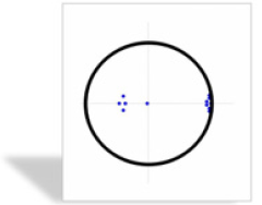
Figure 11: Unit root test.
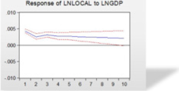
Figure 12: Impulse response.
Principal Component Index System Model: To build a measurement model to measure the vitality of regional economy. Firstly, we establish a scientific, economic vitality index system as the standard of data selection. Secondly, the minimum average difference method is used to screen the data. And the index is initially extracted. Further, the element analysis the method is used to select the main influencing factors. Finally, the comprehensive score of each factor is weighted to give the ranking of urban economic vigor.
The Construction Principle of Index System of Economic Vitality: To select effective data to measure the economic vigor of each city, the following five theory s are given in this paper. The general process is as follows: (Figure 13).

Figure 13: Selection of indicators.
1) Scientific Principle: The selection of measurement indicators must be based on scientific principles and can truly and objectively reflect the influence of various factors on urban economic vitality. The scientific comprehensive index evaluation system of urban economic vigor is the basis of correct analysis and evaluation of regional economic vigor.
2) Principle of Practicability: The construction of evaluation index system is mainly theoretical analysis, which will be affected by the data sources of each index in practical application. Therefore, the availability and reliability of data sources should be ensured in reselecting indicators.
3) Systematic Principle: There should be a certain logical relationship between indicators, which should not only report economic vitality from different aspects.
4) Principle of Comparability: The data of each city should conform to comparability, so the data of each city can be compared horizontally and vertically.
5) Principle of relevance: The comprehensive evaluation index system of local economic vitality should be an organic combination of a series of related indexes.
Data Filtering: The minimum mean square deviation method is used to screen the preliminary data. The observation value is xij, where i is the number of evaluation objects, i.e., the number of cities, j is the number of evaluation indexes, there are 19 cities, each city has 14 indexes. First, the average value and mean square deviation of index j are calculated.
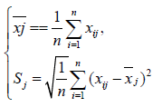
Then the minimum mean square deviation of all indexes is calculated, such as:
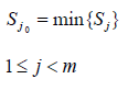
If the minimum mean square deviation is close to 0, then the index be eliminated and calculated in turn.
xj corresponding to Sj can. Finally, nine indexes meeting the requirements can be opted from 14 indexes, namely, local GDP, financial expenditure, the added value of the primary industry, the added value of the tertiary industry, real estate investment, number of college students, population, per capita wage and road traffic noise level.
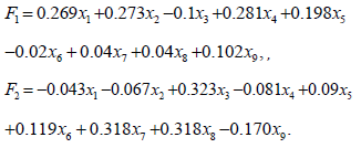
Factor Analysis: Using the factor analysis method, the extracted nine indicators, including 190 sample data from 19 cities in 2009- 2020 are dimensioned down. And then the coefficient matrix is multiplied by the standardized element to calculate the score and find out the factors that have the greatest impact on economic vitality.

Where Fi is the score of the i factor; x1, x2 , xp is the standardized value of the index; the corresponding coefficient is the component score coefficient; The total element score is equal to the weighted arithmetic mean of the scores of each factor, 10 that is

Where is the total factor score, Fi is the score of the first influencing element; Bi is the contribution of the first element, and factor contribution = variance contribution rate/total variance interpretation after the element rotation.
Measurement of the Economic Vitality of Regional Cities: Before measuring the economic vigor of each city, the relationship between variables and element analysis is further verified through the variance of common factors (Table 19). The common factor variance can effectively reflect the strength of its interpretation ability. The larger the common element variance extracted between variables, the stronger the ability to be interpreted by the common factor. Most of the variable factors proposed by the extracted common element variance are explained to a higher degree than 70%. Therefore, the extraction effect is better, the information of the original data loss is less, and the data extracted is more reliable.
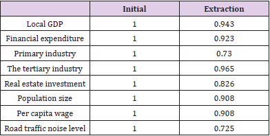
Table 19.Common factor variance extraction.
For the element, whose characteristic root is greater than 1, data analysis is carried out based on SPSS software and two factors are finally obtained, as shown in the table below, with the explanation of total variance. From Table 20, the cumulative variance contribution rate is 73.174%, indicating that the first two factors contain 73.174% of all indicator information (Figure 14). And the extracted information is large and highly representative. Therefore, element analysis is effective in extracting original variable information. From Table 20, the cumulative variance contribution rate is 73.174%, indicating that the first two factors contain 73.174% of all indicator information. And the extracted information is large and highly representative. Therefore, element analysis is effective in extracting original variable information.
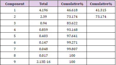
Table 20.Total variance.
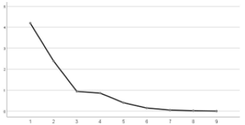
Figure 14: Gravel map.
It can also be seen from the gravel map that the information contributed by the first two factors in the overall influence elements represent that the broken line is relatively steep. And the slope of the broken line is relatively gentle after that, so it can be considered that the two factors extracted are relatively reasonable (Table 21).
It can be seen that the primary industry, tertiary industry, college students, population, and road traffic noise level are factor 1, which reports the level of social production and security. Therefore, element 1 can be named as social production and security factor; local GDP, financial expenditure, real estate investment, and per capita wage are element 2, which reflects the government regulation and control. Therefore, the element two is called the government regulation element. The contribution rate of elements is analyzed by the method of normal maximization variance. And the conversion correlation coefficient is obtained, which shows the correlation of two factors.
It can be seen from Table 22 that in the component transformation matrix, the value of component one has changed, and the value of component two has also changed. It is necessary to extract the component matrix of the factor load matrix.
According to the component score coefficient matrix, local GDP, fiscal expenditure, tertiary industry, tertiary industry, and real estate investment have a positive impact on the ranking; the primary industry hurt the ranking. The expression of each influence factor is given according to Table 23.
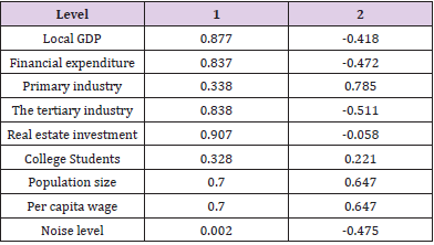
Table 21.Component matrix.
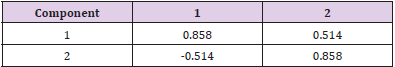
Table 22.Component transformation matrix.
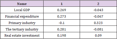
Table 23.Component score coefficient matrix.
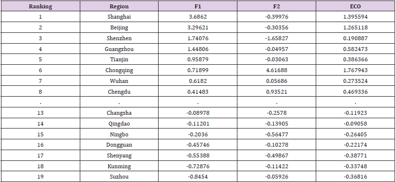
Table 24.Score ranking.
Taking the variance contribution rate of each factor as the weight, the weighted analysis is carried out. After the weighted average, the growth index scores are as follows:
The final weight value of each influencing factor is attained by the factor analysis. And the comprehensive score of each element is obtained by element score weighting function. The element ranking and comprehensive element ranking of each city are shown in Table 24.
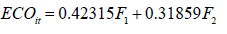
It can be seen from the ranking table that the cities such as Beijing, Shanghai, and Guangzhou rank the second, third and fourth respectively in the ranking, which indicates that the central economic zone of the country has high stability and is not easy to change. The highest ranking is Chongqing. Shenyang is ranked next, and the transfer of its industrial center may be one of the reasons for this outcome. It can be seen from Figure 15 that the ranking of Kunming and Ningbo fluctuates greatly. Considering that the local industrial structure is not obvious enough, it is necessary to strengthen the industrial structure adjustment to improve its economic vitality. Shenyang’s ranking is declining year by year, which may also be related to local policies and development strategies. So, it needs to be noticed in time.
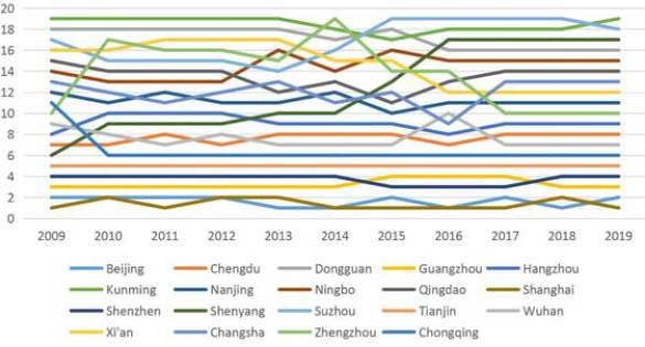
Figure 15: Regional rankings over the past decade.
Comparative Analysis of Factors Affecting Economic Vitality: In the above, according to the factor analysis method, two main elements that affect economic vitality are social production and security elements and government regulation factors, which have a positive correlation with economic vitalities. According to the nine influencing factors opted above, the secondary industry, house price, total retail sales of social goods, number of hospitals, and number of post offices all have a positive impact on the economic vitality. The comparative analysis is made on each element to see if there is any difference.
1) Model Establishment: To test the accuracy of the index system established to measure economic vitality, considering that the individual effect of each index is not observable, and the time effect is not observable, a panel data model is established to test it. And the following model is established:
In the formula, ecoit is a comprehensive index system to measure economic vigor, xit is an independent variable of N rows and K columns. The factors affecting economic vitality can be divided into
a. Social security system: Number of hospitals and Post offices
b. Processing and production: The secondary industry
c. Consumption level: house price, total retail sales of social goods
2) Descriptive Statistics: To analyze the regional economic vitality more specifically, it is necessary to understand the distribution characteristics of each data. Through descriptive statistical analysis of the data, the basic information of each variable (Including sample number, mean value, standard deviation, minimum value and maximum value) is obtained as shown in Table 25. To dissect the regional economic vitality more specifically, it is necessary to understand the distribution characteristics of each data. Through descriptive statistical analysis of the data, the basic information of each variable (Including sample number, mean value, standard deviation, minimum value and maximum value) is obtained as shown in Table 25. It can be seen from Table 25 that the average value of eco is close to 0, indicating that the statistical effect is very good. The fluctuation of the house price is large, which is in line with China’s national conditions. The number of hospitals is quite different, which deserves the attention of local government. The number of post offices is on the high side in some areas, resulting in wastes of resources.
3) Correlation Analysis: Table 25 is the basic situation of the data. After the description and statistics of the data, the correlation analysis of the data is carried out. If the correlation of some indicators is too low, it may lead to the low chi-square significance value, which needs to be screened. Then, the Pearson correlation coefficient is opted to measure the correlation between the variables. If the correlation between the illustrated variables and the explained variables is high, the study of the model is intentional. However, if the correlation between explanatory variables is too high, it may lead to collinearity among variables, which may affect the outcomes of the model. The following studies the correlation between the two variables analyze the correlation between the two variables. And the tests are significant (Figure 16).
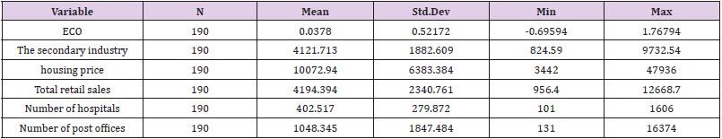
Table 25.Sample description.

Figure 16: ORT development strategy.
From the correlation analysis outcomes of Table 26, it can be concluded that the correlation coefficients between all explanatory variables and the interpreted variables are significant, and there is no strong correlation between the explanatory variables. Therefore, there is no multicollinearity between the explanatory variables. To further study the collinearity among the validation variables. The model was validated by using the VIF test. And the outcomes are shown in Table 27. It can be seen from the table that the VIF value of the explanatory variable and the control variable is less than 5. That is to say, the multicollinearity among the variables is low, which will not have a great impact on the outcomes of the model.
Therefore, the following modeling and regression analysis can be continued. Continue with the residual analysis (Table 28). From the analysis of variance, the F value is far greater than 1, which shows that the differences among the factors are statistically significant. The interaction effect among the factors is more significant. Fixed effect model and mixed model are tested by F test, random effect model and mixed model are tested by BP test, stable effect model and random effect model are tested by the Hausman test, and they are compared (Table 29): According to the model test results, if the p-value corresponding to the F test is 0, less than 0.05, it means that the fixed effect model is due to the mixed model. If the p-value corresponding to the BP test is also 0, less than 0.05, it means that the random effect model is better than the mixed model.
If the p-value corresponding to the Hausman test is 0, it means that the fixed effect model tends to be selected. See Table 30 for regression outcomes of fixed effect model to be opted after inspection. From Table 30, we can see the regression results of the model. And the fixed effect model is opted after the test. The correlation coefficients of the first principal component, the second principal component, the second industry, the house price, the retail sales of social goods, the number of hospitals, and the number of post offices are all positively correlated with Eco. These indicate that they all have a positive impact on economic vitality. From the perspective of economic vigor, the secondary industry, house price, retail sales of social goods, and hospitals, and number of post offices are all positively related to economic vigor. In these variables, when one variable changes, the other variables remain unchanged. Then the economic vigor changes in the same direction. Therefore, it can be further proved that the economic vigor index system constructed in this paper can accurately measure it.
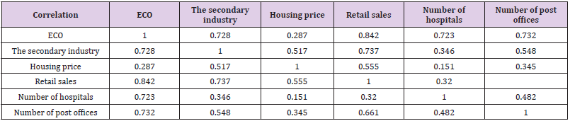
Table 26.Correlation Analysis.
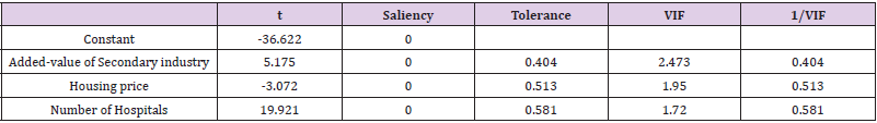
Table 27.VIF test results.
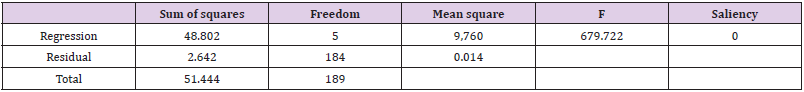
Table 28.VIF test results.

Table 29.Residual analysis results.
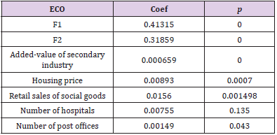
Table 30.Fixed effect regression results.
A Development Plan Based on the Perspective of the Decision-Maker
This section first reviews questions 1 to 3 above and obtains the general universality of the model established in this paper. Finally, according to the outcomes, it proposes measures conducive to improving economic vitality and promoting economic growth.
Conclusion Review
From question 1 to question 3, we can roughly divide the index system of urban economic vitality into indicators of economic growth, indicators of attractiveness to capital and production factors, indicators of employment and residents’ quality of life, indicators of innovation capacity, and indicators of intellectual property protection. Which chose the per capital GDP, fiscal revenue, education and human capital, income levels, employment, innovation, and intellectual property rights protection for data collection, processing, modeling and analysis, and it can provide indicators and economic vitality all remain positive correlation. Therefore, we can dissect from the perspective of the above and advise the sustainable development of the economic vigor of benign and stronger regional competitiveness.
Suggestions on the Benign Sustainable Development of Beijing’s Economic Vitality
Economic vitality includes not only the speed, stability, and outcomes of economic growth, but also the average quality of life of the people, such as the level of education and health standards, as well as the overall progress of the economic structure and social structure (Figure 16). Given the excessive factors affecting economic vitality, we roughly divide the policy into three parts, including optimizing industrial structure (O), rationally controlling investment intensity (R) and technological innovation (T), namely ORT development strategy.
Optimizing the Industrial Structure
a) Vigorously Developing the Tertiary Industry: The third industry is an important indicator of a country’s economic development. And the tertiary industry has the characteristics of less investment, short cycle, quick effect, and high wages of employees. Vigorously developing the tertiary industry can rapidly expand employment fields and jobs, avoid labor surplus, and improve residents’ income. For modern cities, residents not only have material needs but also pursue spiritual level. This growth trend promotes the region to continuously develop new industries to meet the needs of the people, to improve residents and to improve the quality of life. Therefore, we vigorously develop the tertiary industry, which has a significant role in promoting the sustainable development of economic vitality.
b) Strengthening the Development of Primary and Secondary Industries: For the adjustment of Beijing’s economic structure and the promotion of its regional competitiveness, it is necessary to develop the tertiary industry while strengthening the primary industry and expanding the scale of the secondary industry. The first industry is the basic trade of the national economy, strengthening the first industry, and laying the foundation for the development of the second industry and the third industry.
Reasonable Control of Investment: Investment is an important part of GDP but also an element of economic vitality. The growth of investment is of great significance to the promotion of it. In China, investment is mainly divided into a private investment, government investment, and foreign investment. From the perspective of Beijing, as a first-tier city, many foreign enterprises and state- owned enterprises invest in Beijing in various forms. However, the unreasonable investment may cause the princess of resources, leading to an imbalance of social and economic development. Therefore, Beijing should control the scope of investment and improve the efficiency of investment.
Technology innovation: Science and technology are the primary productive forces, and innovation is a force that cannot be ignored to drive economic development. Innovation is conducive to the optimization and transformation of China’s economic growth mode. Economic vitality comes from the sound growth of the economy. We should strengthen the policy support for the investment in science and technology of enterprises, guide the flow of resources such as projects, funds, and talents to enterprises, and establish an innovation support system with enterprises as the main body. Cultivate and develop the next generation Internet, new generation mobile communication, Internet of things, navigation and location services, biomedicine, and other high-tech strategic emerging industries. Accelerate the construction of high-end talents gathering special zone, and actively introduce and cultivate high-end talents.
Model Evaluations
Advantages
The advantages and disadvantages of model factor analysis and panel data model are analyzed.
1) Factor Analysis: Through dimensionality reduction of a variety of influence indicators, the main elements are extracted from the complex elements, and a few factors are used to describe the relationship between many indicators that is, several closely related indicators are classified into the same category, each category of indicators becomes a factor and the economic vitality is measured by a few factors. It simplifies the problem, measures most of the information of it, and gets more scientific and accurate information at the same time.
2) Panel Data Model: Compared with the traditional time series model, the panel data model can provide more data points, increase the degree of freedom of data and reduce the degree of collinearity between explanatory variables, thus improving the effectiveness and accuracy of model estimation; Panel data model is more conducive to reflect the randomness of the gap between individuals. In this paper, panel data model can not only report the information between the given factors, but also report the information of a certain factor through the study of other influencing factors.
Improvements Needed
When using the panel data model to study influence factors, there are some difficulties in variable design and data collection, some errors in factor prediction, and selection difficulties in influence factors; panel data analysis of time series of factors is short, which can only reflect the data characteristics in the short term, not the long-term changes of factors.
Conclusions and Recommendations
This paper establishes three models, namely panel data model (fixed effect model and random effect model), var-vec model and principal component index system construction model. The var-vec model has great generalization. The applicable fields are
a. VaR Based Research on agricultural economic development. Because of its unique ability of testing dynamic fluctuation, AVR can solve the research difficulty of agricultural economy which is greatly affected by seasonal.
b. Oil price evaluation. International oil has been affected by many factors, among which the fluctuation of international political content has a greater impact. Using VAR model can highlight the impact of oil price changes in the short term and make adjustments at any time.
c. The new decline of real estate has an important impact on the national economy. Choosing appropriate research methods will provide a new solution to this kind of problem.
d. Var can also be used for monetary policy analysis to study the long-term and short-term impact of changes in money supply and interest rate on economic fluctuations and their contribution.
Especially in the context of the global epidemic, the economic growth situation and economic growth potential of various countries are issues that need special attention. For a country, the epidemic outbreak may present a point like outbreak trend, and the relationship between the regional epidemic development trend and the regional economy is also inseparable. In the future epidemic prevention and control, we can establish the relevant panel data model and VAR-VEC model and use the relevant local economic indicators to model and analyze how to stabilize the local economy and promote the national economy.
Conflict of Interest
We have no conflict of interests to disclose and the manuscript has been read and approved by all named authors.
Acknowledgement
This work was supported by the Philosophical and Social Sciences Research Project of Hubei Education Department (19Y049) and the Staring Research Foundation for the Ph.D. of Hubei University of Technology (BSQD2019054), Hubei Province, China.
References
- MN Eltony, Mohammad Al‐Awadi (2002) Oil Price Fluctuations and Their Impact on the Macroeconomic Variables of Kuwait: A Case Study Using a VAR Model. International Journal of Energy Research 43(4): 243-153.
- Dimitris K Christopoulos, Miguel A Leon‐Ledesma (2008) Testing for Granger (non-)causality in a time-varying coefficient VAR model. Journal of Forecasting 27(4): 293-303.
- Xiaohong Chen, HAN Wen-qiang, Se Jian (2005) Pricing of Credit Guarantee for Small and Medium Enterprises Based on the VaR Model. Systems Engineering 15(3): 36-41.
- Alsalman Z (2016) Oil price uncertainty and the U.S. stock market analysis based on a GARCH-in- mean VAR model. Energy Economics 59: 251-260.
- Tan, Lu Z (2020) Study on the interaction and relation of society, economy and environment based on PCA–VAR model: As a case study of the Bohai Rim region, China. Ecological Indicators 48: 31-40.
- RD Chen, Dan Cao, Qingyang Yu (2009) Nonlinear VaR model of FX options portfolio under multivariate mixture of normal distributions. Xitong Gongcheng Lilun yu Shijian/System Engineering Theory and Practice 29(12): 65-72.
- Fan K, Guanghai Nie (2013) Study on China's Import and Export Growth Rate Based on VAR Model. Lecture notes in electrical engineering 16(2): 126-134.
- M Trevisan, G Errera, C Vischetti, A Walker (2020) Modelling pesticide leaching in a sandy soil with the VARLEACH model. Agricultural Water Management 44(3): 360-369.
- Ugalde, Anduaga J, Martínez F, Iturrospe A (2020) Novel SHM method to locate damages in substructures based on VARX models. Journal of Physics: Conference Series 628: 12-13.
- Monchen Guido, Sinquin B, Verhaegen M (2020) Recursive Kronecker-Based Vector Autoregressive Identification for Large-Scale Adaptive Optics. IEEE Transactions on Control Systems Technology 32(5): 1-8.
- Varnik, F, L Bocquet, JL Barrat, L Berthier (2002) Shear Localization in a Model Glass. Physical Review Letters 90(9): 095702.
- Wu Wan-Shu, R James Purser, David F Parrish (2020) Three-Dimensional Variational Analysis with Spatially Inhomogeneous Covariances. Monthly Weather Review 130(12): 2905-2916.
- Alexander Gordon J, Alexandre M Baptista (2020) A Comparison of VaR and CVaR Constraints on Portfolio Selection with the Mean-Variance Model. Management Science 50(9): 1261-1273.
- Essery, Richard, John Pomeroy, Jason Parviainen, Pascal Storck (2003) Sublimation of Snow from Coniferous Forests in a Climate Model. Journal of Climate 16(11): 1855-1865.
- John PA Ioannidis, TD Stanley, Hristos Doucouliagos (2020) The Power of Bias in Economics Research. The Economic Journal 127(605): 236-265.
- Lei Sun (2020) Driving Mechanism of the Coordinated Development of Regional Economy-Society- Environment System Based on Grey Incidence Analysis Model—A Case Study of Wanjiang Urban Belt. Modern Economy 11(7): 1226-1244.
- Yuping Hu, Sanying Feng, Jing Zhao (2020) Test for the covariance matrix in time-varying coefficients panel data models with fixed effects. Journal of the Korean Statistical Society 49(2): 159-168.
- DV Rodnyansky (2020) Increasing the Competitiveness of Universities and Research Institutions and Their Impact on the Regional Economy Development. Proceedings of the 2nd International Scientific and Practical Conference“ Modern Management Trends and the Digital Economy: from Regional Development to Global Economic Growth” (MTDE 2020).
- Giorgio Gnecco, Federico Nutarelli, Daniela Selvi (2020) Optimal trade-off between sample size, precision of supervision, and selection probabilities for the unbalanced fixed effects panel data model. Soft Computing 24(21): 15937-15949.
- Oluwasheyi S Oladipo (2020) Migrant Workers' Remittances and Economic Growth: A Time Series Analysis. The Journal of Developing Areas 54(4): 126-173.
- Jong-Suk Han, Jong-Wha Lee (2020) Demographic change, human capital, and economic growth in Korea. Japan & The World Economy 53(2): 79-87.
