 Research Article
Abstract
Magnetic Resonance Imaging (MRI) is a noninvasive medical testing procedure that can help physicians to examine internal body structures and diagnose a variety of disorders, such as tumors. MRI has some advantages over other imaging methods: mainly that there is no risk of being exposed to radiation. As a result of this many researchers from the community of computer vision and machine learning are interested in classifying or segmenting MR images to help physicians perform more detailed investigations and an automatic system for brain tumor detection and classification was proposed. Firstly, brain MR images are preprocessed by using a 5x5 Gaussian filter. Secondly, deep feature extraction was performed by using Alex Net and VGG16 models of pre-trained Convolutional Neural Network (CNN). The obtained feature vectors are combined. These feature vectors were used for MR images classification by Extreme Learning Machines (ELM) classifier. The performances of the proposed methods have been evaluated on three different data sets. Performance parameters used to assess the results are; accuracy, sensitivity, selectivity and Jaccard’s similarity index for tumor detection. The experimental results showed that the proposed system is superior in detecting and classifying brain tumors when compared with other systems.
Keywords: Deep Feature Extraction; ELM; Brain MR Image Classification; Tumor Detection
Abbreviations: MRI: Magnetic Resonance Imaging; CNN: Convolutional Neural Network; ELM: Extreme Learning Machines; PI: Proton Intensity; WHO: World Health Organization; MFCM: Modified Fuzzy C Means; GLCM: Gray Level Co-occurrence Matrix; KSVM: Kernel Support Vector Machines; LBP: Local Binary Pattern; SWT: Stationary Wavelet Transform; GCNN: Growing Convolution Neural Network; SVM: Support Vector Machine; BP: Back Propagation; TCIA: The Cancer Imaging Archive
Introduction
Brain tumors are formed due to the abnormal growth of the cells which become proliferated in an uncontrollable way [1]. Tumors can damage brain cells by pressurizing the skull which consequently begins to negatively affect human health. Brain tumors are encountered with different characteristics and structures. Meningioma develop from the meninges, the membrane covering the brain and spinal cord [2]. Most of meningioma are benign and slow-growing tumors. Glioblastoma is the most common primary malignant brain tumor of all brain tumors. It is also one of the most difficult tumors to treat [3]. The pituitary gland is the region located in the brain base where some hormones are secreted. The benign tumors that develop in the pituitary gland are called pituitary adenomas [4]. Magnetic Resonance Imaging (MRI) is used to examine the structure of the brain tissue [5]. The tumor is composed of various biological tissues; only one protocol cannot give all the information about the tissues of brain. Therefore, MR images obtained on T1, T2 and Proton Intensity (PI) bases need to be considered together to evaluate the state of tumor [6].
Another issue is that the numbers of patients affected by brain tumors have been increasing every year according to the World Health Organization (WHO) data [7]. Yet, brain tumors may progress very rapidly and may have even more negative effects Copyright@ Ali Arı | Biomed J Sci & Tech Res | BJSTR. MS.ID.004201. Volume 25- Issue 3 DOI: 10.26717/BJSTR.2020.25.004201 19138 on human health. Therefore, the evaluation of images should be done quickly as it is vitally important in cancer diagnosis and treatment planning. Manual examination by experts could be time consuming, therefore, an alternative option is a dedicated automated system that helps physicians in their diagnosis and thereby speed up the treatment process. There are many computerassisted automatic detection and diagnosis systems in literature [8]. Karim et al. [9] have presented a new method by combining the Gauss Mixture Model (GMM) and the Modified Fuzzy C Means (MFCM) algorithm for tumor detection from brain MR images. Duan et al. [10] have proposed a new method for performing brain MR image segmentation. This method involved low pass filtering, segmentation using a threshold value and morphological process. Ahmadav et al. [11] have proposed a method in which the features from brain MR images were extracted by using wavelet transform. Random Forest classifier was used for classification of MR images as tumor or non-tumor.
Kadam et al. [12], have proposed a method in which the features were extracted by Gray Level Co-occurrence Matrix (GLCM). Kernel Support Vector Machines (KSVM) classifier was used for classifying MR images as tumor or non-tumor. Abbasi et al. [13] have introduced a brain tumor detection method which automatically estimates tumors from volumetric MR images. The images were preprocessed using a histogram equalization method. Those structures that could be considered as tumors were segmented from the images. Some of the features extracted from these structures that have the potential of being tumors. By using the Local Binary Pattern (LBP) method along with these features, a variety of classifiers are selected, and the performances of these classifiers were compared. Mittal et al. [14] the Stationary Wavelet Transform (SWT) and novel Growing Convolution Neural Network (GCNN) approaches are used in the recommended method. This study mainly aims to reach higher levels of precision in comparison to that of the conventional systems. Support Vector Machine (SVM) and Convolution Neural Network (CNN) are compared and analyzed. Consequently, it is seen that the suggested method is much better than SVM and CNN from the point of various performance criteria such as precision, PSNR, MSE etc. Sajjad et al. [15] a newly developed system which classifies brain tumors on the basis of convolutional neural network (CNN) is introduced. The experimental results which is obtained from both enhanced and original data indicate that the performance of the method is clearly superior to the current techniques. Habib et al. [16], particularly focuses on modelling the distortive activity of malignant tumors.
They suggested a dynamical profile of heterotypic and holotype attractor chemicals depending on the patio-temporal patterns which are obtained from an experiment on multicellular brain tumor spheroids. A newly developed, theory based, and computational approach was presented in order to analyze a mathematical tumor model which includes several coupled reactions like diffusion reactions which state chemotactic and hepatotactic behaviors of cells.
In this study, brain MR images were classified in accordance with tumor types. The tumors are segmented using a threshold value defined by add hook. The algorithm starts with filtering out the high frequency components on the images that may be considered as noise using a Gaussian filter. Then, pre-trained CNN models were used to extract features from the images. These are the feature vectors extracted from fc6 and fc7 layers of Alex Net and Vgg16 models. Then, the combinations of these vectors were fed to ELM classifiers. The tumors were segmented from the classified images with a dedicated threshold value set by trial and error. Finally, morphological operations and tumor masking operations were applied to eliminate mis-segmented pixels in the segmented images. The organization of this paper is as follows. In the next section, the methodology will be introduced. In section 3, the data sets used in this study will be explained. The experimental studies and the results will be explained in section 4. The study will be concluded in section 5.
Preliminaries
An automatic computer assisted system was designed for the detection of brain tumors. The proposed system was tested on MR images. Tumor detection from MR images is more efficient due to high contrast and spatial resolution, and also healthier due to low radiation. MR images provide information about the location and size of the brain tumor, but types of the tumors cannot be directly categorized from these images. In this case, experts wait for the result of the biopsy. The aim of the proposed system was to classify brain tumors according to their types using MR images and to determine the brain tumor. The proposed system consists of five main steps; pre-processing, extraction of deep features, concatenation of deep features, classification of feature vectors and detection of brain tumors. Figure 1 shows the operating principle of the proposed method. The methodology was given in the following sections.
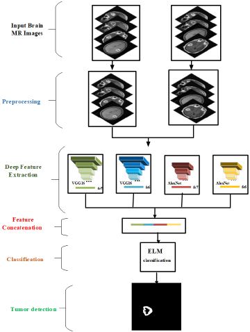
Figure 1: Operating principle of the proposed method.
Pre-Processing
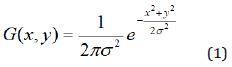
Depending on the application, a variety of linear, non-linear, fixed, adaptive or pixel-based pre-processing methods are usually employed before classification to enhance the sensitivity [7,17]. In some conditions where the differentiation between normal and abnormal tissue is complex due to high noise level, experts may naturally make mistakes in interpretation. On the other hand, minor differences between normal and abnormal tissues can also be masked by noise. Therefore, it is necessary to remove the possible noises with preprocessing MR images. Also, the enhancement in the visual quality of the image provides great benefits to experts. In this study, MR images were pre-processed with a 5 × 5 Gaussian filter using Matlab environment. The used filter is given in Eq. 1, where σ represents the bandwidth of the filter.
Feature Extraction With Pre-Trained CNN Models
Two pre-trained CNN models, Alex Net and VGG16, were used in this study for feature extraction. Alex Net is known as the first deep CNN structure which consists of twenty-five layers, eight of which contribute to learning by adjusting weights. Five of these layers are convolution layers while remaining three are fully connected. In Alex Net architecture, max-pooling layers come after the convolution layers, and convolution layers use varying kernel sizes [18]. Another deep CNN model is the VGG16 model proposed by Simonyan et al. [19]. The VGG16 model consists of 41 layers, 16 layers of which have adjustable weights. These layers are composed of 13 convolution and 3 fully connected layers. The VGG16 model uses only 3 × 3 dimensional kernels in all layers of convolution. Similar to Alex Net, max-pooling layers follow the convolution layers [18,19]. Activations (fc6, fc7) in the first and second fully connected layers are used to extract feature vectors. fc6 and fc7 vectors contain in total 4096 features.
Extreme Learning Machine
The Extreme Learning Machine (ELM) was firstly designed by Huang et al. [20]. ELM is a single hidden layered feed forward neural network whose input weights are calculated randomly, and output weights are calculated analytically [20-22]. This approach has several advantages over conventional learning algorithms like Back Propagation (BP) [23]. A sample ELM model is shown in Figure 2. There are different types of activation functions in ELM such as sigmoid, hard-limited, triangular and radial basis. In this study, activation function was determined as sigmoid after some trial and error steps. 10-k cross validation test was used and the number of neuron in hidden layer is 10.000.
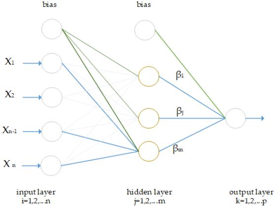
Figure 2: Single hidden layered feed forwarded neural network.
Segmentation
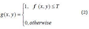
The segmentation process was performed to separate brain texture from other textures in the MR images. Thus, structures such as skulls, backgrounds, scalps and eyes were removed from the MR images. The basic principles of segmentation algorithm rely on region enlargement, deformable templates, clustering with thresholding and pattern recognition techniques. In this study, the structures that might be tumors were segmented by a threshold value determined as described in Eq. (2).
Datasets
Three data sets which are open access related to brain MR images were used in this study. The first data set was RIDER. The Cancer Imaging Archive (TCIA) organized RIDER brain image data that consists of 126 patients in which each case per patient comprises of multiple studies. Data was collected from Henry Ford Hospital (RETRO) and TJU Institute. Along with the MRI data, information about the patients suffering from different stages of brain diseases was obtained i.e., Astrocytoma, GBM, and Oligodendro gliomas along with race (white, black). Pathologists assign grades 1, 2, 3, 4 dues to the survival rate of disease in which 41 images belong to grade 2, 36 are from grade 1, 26 images belong to grade 3 and 23 are from grade 4 tumor [6,24]. The second data set was Figshare. The Figshare brain tumor dataset [25] contains 3064 T1-weighted contrast-enhanced images from 233 patients with three kinds of brain tumors: meningioma (708 slices), glioma (1426 slices), and pituitary tumor (930 slices).
The third data set was REMBRANDT. It belongs to the TCIA. All images are in DICOM file format. Images in archive were organized according to disease and imaging method. All images of the REMBRANDT dataset were digitized at a resolution of 256 x 256 pixels and at 16 bit gray level. Each section has a thickness of 5 mm. This data set contains 33 patient images. There are 20 MR section images of each patient on average in axial, sagittal and coronal planes separately [26].
Experimental Studies and Results
Experiments were conducted to test the performance of the proposed system. A computer with Intel Core i5-4810 CPU and 8 GB memory is used in the experiments and programs are written in MATLAB 2017-b environment.
Classification Results
Brain MR Images were resized to 227 × 227 and 224 × 224 sizes respectively to use for Alex Net and VGG16 models. The features of brain MR images were removed from the layers fc6 and fc7. Each CNN model produces a feature vector of size 4096. Later, these vectors were combined. Tables 1-4 show the classification accuracies obtained with the ELM. The feature vectors generated by the layers fc6 and fc7 of the Alex Net and VGG16 architectures with various combinations. Tables 1-3 present the combined feature vectors, accuracy of classification results and length of feature vectors, respectively. Table 1 presents the results obtained for RIDER data set. Table 1 indicates that all deep feature combinations produce acceptable accuracy and the combination of Alex Net fc6 and VGG16 fc6 feature sets provides the highest accuracy. The highest accuracy is 99.00% and number of features are 8192. The second highest accuracy value was 98.90% and it was obtained for feature combinations of Alex Net fc6, Alex Net fc7, VGG16 fc6, VGG16 fc7 and the feature number was 16384. The calculated lowest accuracy was 97.90% from the feature combinations of Alex Net fc6 and Alex Net fc7 and the feature number was 8192.
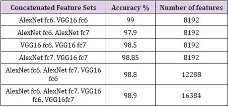
Table 1: Obtained accuracies for various combinations of feature sets for RIDER dataset.
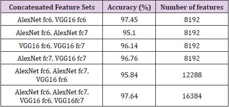
Table 2: Obtained accuracies for various combinations of feature sets for Figshare dataset.
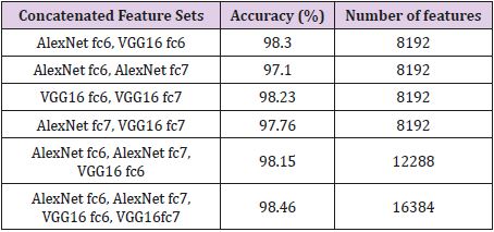
Table 3: Obtained accuracies for various combinations of feature sets for REMBREDANT dataset.
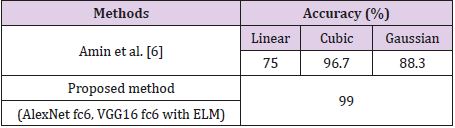
Table 4: Comparison of proposed method with existing method (%).
Table 2 shows the results obtained for the Figshare data set. It is seen that the combination of all feature sets produced the highest accuracy of 97.64% for the Figshare data set. Feature set combination of Alex Net fc6 and VGG16 fc6 was also the second highest accuracy. The lowest accuracy was obtained as 95.10% from the feature set combination of Alex Net fc6 and Alex Net fc7. Table 3 shows the results for REMBREDANT data set. Table 3 shows that all deep feature combinations produce acceptable accuracy and the combination of all feature sets provides the highest accuracy. The highest accuracy was 98.46% and the feature numbers was 16384. The second highest accuracy was 98.30% for the feature combinations of Alex Net fc6 and VGG16 fc6, and the feature numbers was 8192. The lowest accuracy was calculated as 97.10% from the feature combinations of Alex Net fc6 and Alex Net fc7, and the number of features was 8192. The highest accuracy rates obtained for each data set were compared with other methods in the literature. In Table 4, proposed method was compared with Amin et al.’s method that used RIDER data set. As seen in Table 4, our proposed method is superior then Amin’s method with 10- fold cross validation [6]. Table 5 compares the proposed method with the Jun Cheng et al. who used Figshare dataset. As seen in Table 5, the success achieved by Jun Cheng et al. was 94.68%. This performance ratio was less than the success we have achieved from our proposed deep feature combinations. In Table 6, proposed method was compared with Kazdal et al. who used REMBREDANT data set. As shown in Table 6, the classification performance obtained by Kazdal et al. was 84.26%. This performance ratio was less than the success we have achieved from proposed deep feature combinations.
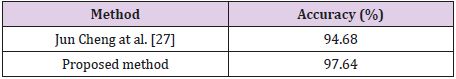
Table 5: Comparison of proposed method with existing method (%).

Table 6: Comparison of proposed method with existing method (%).
Segmentation Results
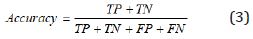
During the segmentation phase of the image, global thresholding was used, and a threshold value was selected for this. When the pixel value of interested region was less than the threshold value, it was ignored, and the image was transformed into binary image. Thresholding process gives faster results than the methods performing segmentation by using generally more than one feature of the image. Since brightness, especially in the majority of biomedical images, is a distinctive feature in terms of segmentation, it becomes an application area where the thresholding process can be used. After the thresholding process, morphological operations and windowing technique were used. When the performance evaluation based on accuracy, sensitivity and specificity were performed, it was observed that the best threshold was T = 155. The performance values in determining the threshold were shown in Table 7. The rows show the tested threshold values while the columns show the calculated numerical performance measures in Table 7. As can be seen from Table 7, the accuracy, sensitivity and specificity values were calculated as 0.3213, 0.1640, 10,817 for T=140, 0.6336, 0.0437, 3110 for T=145; 0.7073, 0.0107, 1146 for T=150, 0.8410, 0.0030, 235 for T=155 and 0.6970, 0.0078, 513 for T=160, respectively. For comparison of ground truth segmented images with our segmented images, accuracy, sensitivity, specificity and values of Jaccard’s Index of Similarity parameters were used. These parameters are given in Eq. (3) to (6).
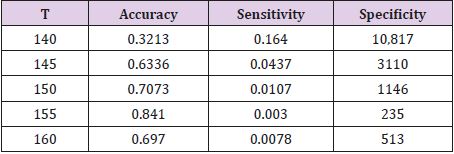
Table 7: The results of optimal threshold values for tumor detection.


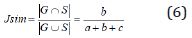
In Eq. (3), to (5), TP refers the correct location of tumor pixels, TN refers to non-tumor pixels. FP refers the perception of healthy pixels as tumor tissue pixels. FN refers the undetected tumor pixels. In Eq. 6, Jsim parameter gives Jaccard’s index of similarity. It takes values between [0, 1]. If the images are completely similar, Jsim parameter is equal to 1. If there is no similarity between the images, the parameter becomes 0. The results of each process performed during brain tumor detection were indicated in Figure 3. In the first column, brain MR images, in the second column, images as a result of pre-processing, in the third column, images formed as a result of thresholding, in the fourth column, images as a result of morphological operations and masking, in the fifth column, images based on the result of Jaccard’s similarity are included and the pink parts in the images show that there is a missing area when compared to actual binary tumor images and the green parts show that there is much area. Rows represent brain MR images of RIDER, Figshare, and REMBREDANT data sets, respectively. When the Figure 3 is reviewed visually, it is seen that tumor regions have been successfully segmented close to real. When the tumor detection results of the data sets were examined, the tumor performance was on the acceptable level for three data sets. It was seen that the best success in tumor detection was obtained from RIDER data set.
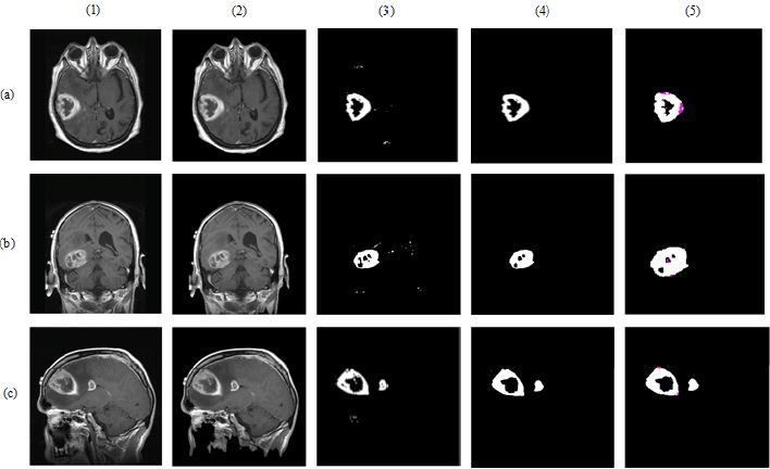
Figure 3: The Stages of Tumor Detection.
The results given in Table 8 confirm the visual evaluation. While rows indicate the names of the data sets, columns present the calculated numerical performance criteria in Table 8. As seen from Table 8, the values of accuracy, sensitivity, specificity and Jaccard’s index calculated for RIDER data set were 98.91%, 98.15%, 98.20%, 98.52% respectively, while these values were 97.44%, 97.12%, 97.54%, 96.88% for Figshare data set and 97.90%, 96.53%, 97.19% and 97.23% for REMBREDANT data set.
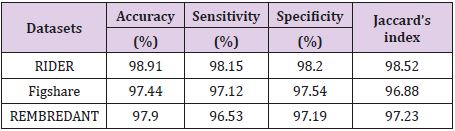
Table 8: The results of parameters for segmentation.
Conclusion
Firstly, the effects of combined deep features on image classification have been examined in this article. In other words, the best way to combine deep feature sets in the task of classifying brain MR images is investigated. Two pre-trained CNN models were used to extract feature vectors from three different data sets. Results indicate that proposed brain tumor classification yields better accuracy in comparison to those available in the literature for the selected datasets. In future studies, we are planning to investigate the classification effect of feature combination of early layers. In this study, tumor detection from brain MR images was performed with segmentation by means of thresholding, followed by morphological operations. In the future studies, it is planned to perform tumor detection with new segmentation techniques.
Highlights
1. This study applies convolutional neural network to brain MRI images classification and tumor detection by using threshold value.
2. It employs a pre-trained CNN model for feature extraction.
3. Extreme Learning Machines (ELM) classifier is employed to classify brain MRI images.
4. The best evaluated classification performance achieved 99% for RIDER dataset.
Funding
This study was not funded by any organization
Conflict of Interest
No potential conflict of interest was reported by the authors.
Ethical Approval
This article does not contain any studies with human participants or animals performed by any of the authors.
References
- McFaline-Figueroa JR, Lee EQ (2018) Brain Tumors. The American Journal of Medicine 131(8): 874-882.
- Zweckberger K, Unterberg AW, Schick U (2013) Pre-chiasmatic transection of the optic nerve can save contralateral vision in patients with optic nerve sheath meningioms. Clinical Neurology and Neurosurgery 115(12): 2426-2431.
- Lagman C, Sheppard JP, Romiyo P, Nguyen T, Prashant GN, et al. (2018) Risk factors for platelet transfusion in glioblastoma surgery. Journal of Clinical Neuroscience 50: 93-97.
- Knaus CM, Patronas NJ, Papadakis GZ, Short TK, Smirniotopoulos JG (2016) Multiple Endocrine Neoplasia, Type 1: Imaging Solutions to Clinical Questions. Current Problems in Diagnostic Radiology 45(4): 278-283.
- Zeng K, Zheng H, Cai C, Yang Y, Zhang K, et al. (2018) Simultaneous single- and multi-contrast super-resolution for brain MRI images based on a convolutional neural network. Computers in Biology and Medicine 99(1): 133-141.
- Amin J, Sharif M, Yasmin M, Fernandes SL (2017) A distinctive approach in brain tumor detection and classification using MRI. Pattern Recognition Letters.
- Louis DN, Perry A, Reifenberger G, von Deimling A, Figarella-Branger D, et al. (2016) The 2016 World Health Organization Classification of Tumors of the Central Nervous System: A summary. Acta Neuropathol 131(6): 803-820.
- Ari A, Alpaslan N, Hanbay D, Beyin MR (2015) Computer Aided Tumor Diagnosis System from Medical Products, National Congress of Medical Technologies, Bodrum Turkey pp. 15-17.
- Karim K, Mohamed M (2014) Image segmentation by Gaussian mixture models and modified FCM algorithm. The International Arab Journal of Information Technology 11(1): 11-17.
- Duan Y, Chang H, Huang W, Zhou J, Lu Z, et al. (2015) The L0 regularized mumford-shah model for bias correction and segmentation of medical images. IEEE Transactions on Image Processing 24(11): 3927-3938.
- Ahmadvand A, Kabiri P (2016) Multispectral MRI image segmentation using Markov random field model. Signal Image and Video Processing 10(2): 251-258.
- Kadam M, Dhole A (2017) Brain tumor detection using GLCM with the help of KSVM. International J Engineering Tech Res 7(2): 2454-4698.
- Abbasi S, Tajeripour F (2017) Detection of brain tumor in 3D MRI images using local binary patterns and histogram orientation gradient. Neurocomputing 219(5): 526-535.
- Mittal M, Goyal LM, Kaur S, Kaur I, Verma A, et al. (2019) Deep learning based enhanced tumor segmentation approach for MR brain images. Applied Soft Computing Journal 78: 346-354.
- Sajjad M, Khan S, Muhammad K, Wu W, Ullah A, et al. (2019) Multi-grade brain tumor classification using deep CNN with extensive data augmentation. Journal of Computational Science 30: 174-182.
- Habib S, Molina-Paris C, Deisboeck TS (2003) Complex dynamics of tumors: Modeling an emerging brain tumor system with coupled reaction-diffusion equations. Physica A 327(3-4): 501-524.
- Hoyosa FT, Landrove MM (2012) 3-D in vivo brain tumor geometry study by scaling analysis. Physica A 391(4): 1195-1206.
- Krizhevsky A, Sutskever I, Hinton GE (2012) ImageNet classification with deep convolutional neural networks. in Advances in Neural Information Processing Systems pp. 1097-1105.
- Simonyan K, Zisserman A (2014) Very Deep Convolutional Networks for Large-Scale Image Recognition. Computing Research Repository (CoRR) pp. 1409-1556.
- Tian H, Meng B, Wang S (2010) Day-ahead electricity price prediction based on multiple ELM. Chinese Control and Decision Conference, 241–244, Xuzhou, China.
- Deng W, Zheng Q, Chen L (2009) Real-Time Collaborative Filtering Using Extreme Learning Machine. IEEE/WIC/ACM International Joint Conference on Web Intelligence and Intelligent Agent Technology pp. 466-473, Milan, Italy.
- Arı B, Şengür A, Arı A (2016) Local Receptive Fields Extreme Learning Machine for Apricot Leaf Recognition. International Conference on Artificial Intelligence and Data Processing (IDAP16), Malatya, Turkey.
- Milačić L, Jović S, Vujović T, Miljković J (2017) Application of artificial neural network with extreme learning machine for economic growth estimation. Physica A 465(1): 285-288.
- Sam A, Beichel R, Bidaut L, Clarke L, Croft B, et al. (2018) RIDER(Reference Database to Evaluate Response) Committee Combined Report, 9/25/2008 Sponsored by NIH, NCI, CIP, ITDB Causes of and Methods for Estimating/Ameliorating Variance in the Evaluation of Tumor Change in Response-to Therapy.
- https://figshare.com/articles/brain_tumor_dataset/1512427, online access: 15.04.2018.
- National Cancer Institute http://www.cancerimagingarchive.net/ online access: 10.03.2018.
- Cheng J, Yang W, Huang M, Huang W, Jiang U, et al. (2016) Retrieval of Brain Tumors by Adaptive Spatial Pooling and Fisher Vector Representation, PloS one.
- Kazdal S, Dogan B, Camurcu AY (2015) Computer-Aided Detection Of Brain Tumors Using Image Processing Techniques. Signal Processing And Comm. Applications Conference (SIU), pp. 863- 866.
