 Research Article
Abstract
Evolutionary adaptation and fixation are distinct physical processes. These processes may or may not be occurring together in an evolutionary process. In this study, we demonstrate both mathematically and empirically that fixation is not necessary for adaptation (improvement in fitness) to occur. And if fixation is required for adaptation, it slows the evolutionary adaptation process. The mathematics of a particular fixation process, the Lenski E. coli long term evolution experiment is derived with a numerical solution and this solution is used to analyze smaller and larger carrying capacity environments.
Keywords: Evolution; Fixation; Adaptation; Mathematical Model
Introduction
Any understanding of an evolutionary process requires the understanding of the particular components that make up that evolutionary process. Darwin wrote about these evolutionary processes in his book, “On the Origin of Species”[1]. From this text, we get a particular quote that describes these processes: “For it should be remembered that the competition will generally be most severe between those forms which are most nearly related to each other in habits, constitution and structure. Hence all the intermediate forms between the earlier and later states, that is between the less and more improved state of a species, as well as the original parent-species itself, will generally tend to become extinct. So it probably will be with many whole collateral lines of descent, which will be conquered by later and improved lines of descent. If, however, the modified offspring of a species get into some distinct country, or become quickly adapted to some quite new station, in which child and parent do not come into competition, both may continue to exist.” Darwin recognized that two processes can occur during evolution, competition (what Darwin also calls the struggle for existence) and adaptation. Many papers have been written about the mathematics of competition. Some of the many examples were written by Haldane et al. [2-5]. Here, we will address both the mathematics of competition and the mathematics of adaptation. In this paper, we consider a particular experimental evolutionary model, the Lenski E. coli long term evolution experiment (LTEE) [6] and the particular evolutionary components which cause the experiment to act in its manner. And to address why it takes so many generations for each fixation and adaptation step. A model for fixation was presented in the following paper BH Good, et al. and edited by Richard Lenski where they discuss these issues [7].
Their model doesn’t directly model the LTEE, however, we will present the mathematical model for fixation for this particular experiment. We will also show the distinction between fixation and adaptation. The mathematical model for fixation for the LTEE presents different physical conditions than standard fixation models such as presented by Haldane, Kimura, and Good. Haldane in his The Cost of Natural Selection [2] paper presents a model for a part of the selection process occurring in the LTEE. But this model does not include the selection process that the Lenski team imposes daily on their populations. To understand what is being done, one must consider how the LTEE is designed. The LTEE is designed to operate in 10ml test tubes using a DM25 glucose solution which supports about 5 x 10⁷ cells per ml of solution [8] or about 5 x 10⁸ cells in a 10ml tube before the glucose is exhausted. For a typical day in the experiment, they grow these 5 x 10⁸ cells and then the glucose must be replenished. This is done by taking 1% (0.1ml) of the day’s growth and using this as a starter in a fresh 10ml tube for the next day’s growth which allows for 6 to 7 doublings (generations) of his populations.
This “sampling” of the previous day’s grow to start the new day’s growth is a type of bottleneck effect. This type of sampling process is described by the hypergeometic distribution [9] and is random sampling which should not change the “evolutionary” direction. On the other hand, if the bottleneck was caused by a directional selection pressure such as allowing 99% of the days’ population to starve to death, the remaining variants would be the members most adapted to those starvation conditions. This concept would have significance, for example, in treating infections. If an antibiotic was only successful in killing 99% of the bacteria in an infection, the remaining 1% could grow without competing with less fit variants in the population. This would most likely accelerate the evolutionary process of drug-resistance.
In this study, we make the simplifying assumption that the distribution of variants in the entire 10ml test tube is identical to the distribution of variants in the 0.1ml sample. The other selection process is the natural selection process that occurs as the different variants replicate where the more fit variant ultimately substitutes for the less fit variants over generations. This is due to the differences in the relative fitness of the different variants in the population. These two selection processes must be combined to correctly describe the fixation process in the LTEE. But the fixation process does not describe the adaptation process. Adaptation (an improvement in fitness) occurs when another beneficial mutation occurs on the more fit variant. The improvement in fitness of a particular variant is dependent on the absolute fitness of that variant to replicate because the random trial for improvement in fitness is the replication and the frequency at which the beneficial mutation occurs is given by the mutation rate. This is a binomial probability problem, that is, does the beneficial mutation occur or does it not occur with that replication. The mathematical model to describe this part of the evolutionary process is given by the mathematics of random mutation and natural selection [10]. The probability of that beneficial mutation occurring on the more fit variant is dependent on the number of replications of that variant. This value will be tabulated in the mathematical model of fixation. The key point to understand in the evolutionary process is that fixation is not a requirement for adaptation. If the carrying capacity of the environment is sufficient to allow for the number of replications required to give a reasonable probability of a beneficial mutation occurring on some variant, then fixation is not needed for adaptation. This will be demonstrated in the following analysis.
Methods
There are several cycles that are occurring in the LTEE. One cycle is the daily growth from its initial 1% starting population from the previous day’s growth (or the single more fit variant on day 1 and the rest of starting population consisting of less fit variants) give 6-7 doublings and the complete consumption of that day’s glucose. A second cycle consists of the number of generations necessary for the more fit variant of the population to fix, driving the less fit variant to extinction. A third cycle is the amplification cycle of the more fit variant where the number of the replications of that variant increases to improve the probability of a beneficial mutation occurring on that variant. A numerical solution to this process is derived including all multiple daily growth cycles, a single cycle of fixation and a single cycle of amplification. This gives the mathematics for a single evolutionary step. The population is assumed to consist of two variants, a more fit variant and less fit variants. The total population at the start of this cycle is assumed to be 1% of the total carrying capacity of the solution from the previous day’s growth (or a single more fit member and the rest of the population consisting of less fit members at generation 1).
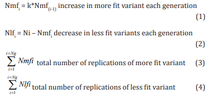
For the actual empirical experiment where 10ml tubes are used, the total growth for the day will be 5 x 10⁸ cells (minus the initial 5 x 10⁶ cells to start that day’s growth). Those starter cells for the day are allowed to double until they reach a population that which if doubled would exceed 5 x 10⁸ cells and that increase in population is limited to 5 x 10⁸ cells. Two other theoretical cases are evaluated based on scaling the experiment down to 1ml daily volume and scaled up to 100ml daily volume. 1% of those volumes are used as starter populations for the next day’s growth. The daily generation population sizes for the 10ml, 1ml, 100ml experiments are tabulated below the Table 1: The computation of the rate of fixation for the LTEE cannot be done with the usual algebraic fixation models. This is because a discontinuity is introduced into the population with the removal of 99% of the population on a daily basis (about every 6½ generations). It might be possible to do a sequence of algebraic equations which describe the rate of fixation for a single day using the final population values from one day as the starting values for the next day, but a much simpler approach is used. A numerical model is developed which computes population values as the fixation process is occurring on a generation by generation basis. This numerical method is described in the next paragraph. The total population at each step is the sum of the more fit and less fit variants. On the beginning of the first day of the process, it is assumed that there is only a single member of the more fit variant. At each generation, the more fit variant increases in number where that number is computed by a replication weight factor. If that weight factor is 2, that means that variant is doubling in number every generation. The final day’s growth for the more fit variant is reduced to account for the fact that the entire population is not doubling. The amount of reduction is computed by taking the final day’s growth and dividing that value by the population size if it were able to double. So, for example, for the 10ml case, that reduction in growth would be computed as (5 x 10⁸ / 6.4 x 10⁸ ) = 0.78125.
The population size for the less fit variant is computed by subtracting the population of more fit variants from the total population at that step. The starting population for the next day’s growth is computed by taking 1% of the final day’s growth to simulate the bottleneck effect from the actual experiment. It is assumed that the relative frequency of the variants is the same as in the final day’s growth. If in any generation, when the population of the more fit variant equals or exceeds the total population size for that generation, fixation has happened. When the more fit variant is fixed in the population, the less fit variant has gone extinct. This daily cyclical process is continued until the less fit variant goes to zero and fixation of the more fit variant has occurred. The total number of replications of the more fit variant is calculated since that number determines the probability of the next beneficial mutation occurring. The total number of replications of the less fit variant is also calculated to demonstrate what Haldane calls “the cost of natural selection”.
The calculation is performed for the 3 different volume tubes, 10ml (the actual experiment condition), and scaled up or down, 1ml and 100ml (theoretical alternate carrying capacity environments) (Figure 1). The replication weight factor is identified which would give fixation in about 500 generations for the actual experimental conditions and for different values of the weight factor to determine how this would affect the rate of fixation and amplification of the more fit variant. This daily cyclical process is continued until the less fit variant goes to zero and fixation of the more fit variant has occurred. The total number of replications of the more fit variant is calculated since that number determines the probability of the next beneficial mutation occurring. The total number of replications of the less fit variant is also calculated to demonstrate what Haldane calls “the cost of natural selection”. The calculation is performed for the 3 different volume tubes, 10ml (the actual experiment condition), and scaled up or down, 1ml and 100ml (theoretical alternate carrying capacity environments) (Figure 2). The replication weight factor is identified which would give fixation in about 500 generations for the actual experimental conditions and for different values of the weight factor to determine how this would affect the rate of fixation and amplification of the more fit variant.
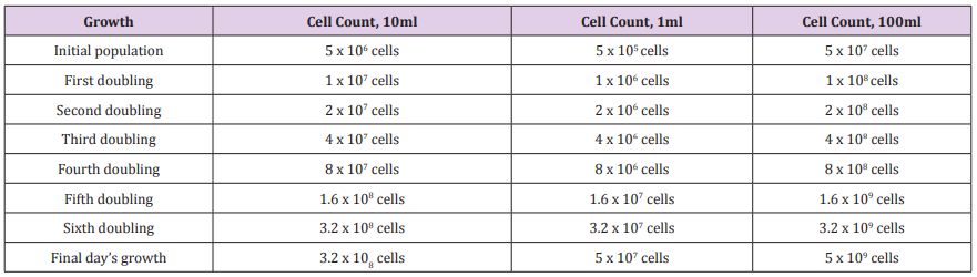
Table 1: Daily cell growth for 10ml, 1ml, and 100ml experiments.
Definition of Variables
Ni total population size at step “i”
Nmfi more fit population size at step “i”
Nlfi less fit population size at step “i”
k replication weight factor for the more fit variant (if k=2, the more fit variant doubles every time the total population doubles)
Ng number of generations Equations used at each step of calculation:
For the last (partial) generation of the day, the value for the more fit variant is reduced by a factor of (50/64) to take into account that a full doubling of the population is not occurring. In addition, the number of the more fit variant is reduced by a factor of (1/100) to take into account the removal of 99% of the population at the start of the next day’s growth cycle (Figure 3). The values for the more and less fit variants are then computed on a generation by generation basis until either the more fit variant equals the total population for that generation, or 500 generations are reached.
Results
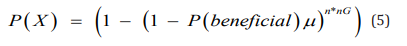
The following tables give the number of generations for fixation (if it occurs) for the three tube sizes(1ml, 10ml, and 100ml), and the number of replications of the more fit and less fit variants at the time of fixation (or at 500 generations if fixation does not occur). Table 2, Table 3 & Table 4 what the above calculations demonstrate is that as the fixation process is occurring, the number of replications of the more fit variant is increasing (Table 1). As the number of replications of the more fit variant increase, the probability of a beneficial mutation occurring on one of its members is also increasing. It was shown in reference [10] that the probability of a beneficial mutation which would improve fitness to some member of a variant subject to only a single selection pressure is: What the above calculations demonstrate is that as the fixation process is occurring, the number of replications of the more fit variant is increasing. As the number of replications of the more fit variant increase, the probability of a beneficial mutation occurring on one of its members is also increasing. It was shown in reference [10] that the probability of a beneficial mutation which would improve fitness to some member of a variant subject to only a single selection is:
Where,
P(X) is the probability of a beneficial mutation occurring,
P(beneficial) is the probability that the mutation that occurs at the particular site is the beneficial mutation,
μ is the mutation rate, and
n*nG is the total number of replications.
Note that n*nG is assuming a constant population size that is replicating for nG generations, but this term can be generalized to a summation of all replications over all generations without altering the underlying P(X). The fixation curve, the total number of replications of the more fit variant and the probability curve as a function of generations for a beneficial mutation to occur is displayed below for the case of the 10ml tube, k=1.894 experiment (Table 2). Note, the curves are cropped between 25 and 345 generations because the curves are essentially not changing during this interval (Figure 1,2 & 3).
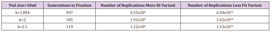
Table 2: Generations to fixation and total number of replications for 10ml experiment and several values of k.

Table 3: Generations to fixation and total number of replications for 10ml experiment and several values of k.
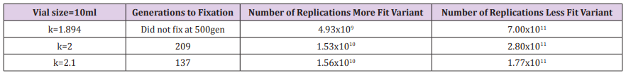
Table 4: Generations to fixation and total number of replications for 100ml experiment and several values of k.
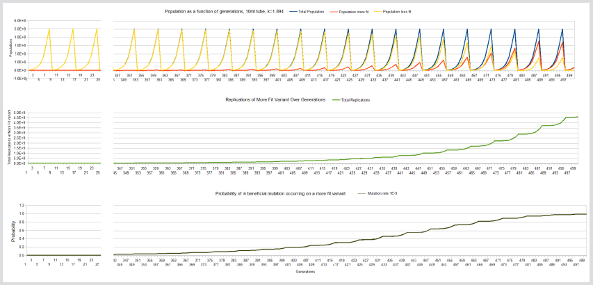
Figure 1: Fixation, total replication more fit variant and probability a beneficial mutation will occur on the more fit variant curves, 10ml tube, k=1.894.
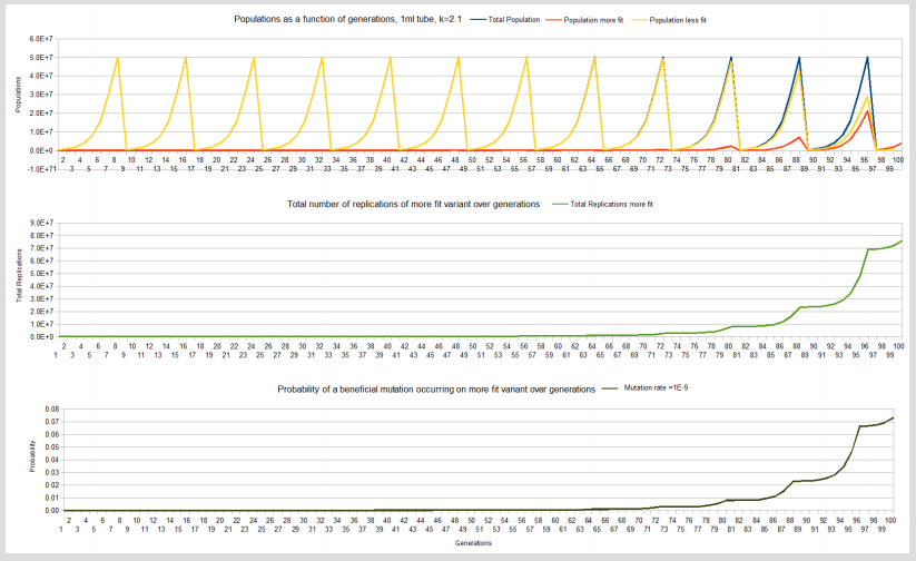
Figure 2: Fixation, total replication more fit variant and probability a beneficial mutation willoccur on the more fit variant curves, 1ml tube, k=2.1
Note: The following curves are for the 1ml tube, k=2.1 experiments.
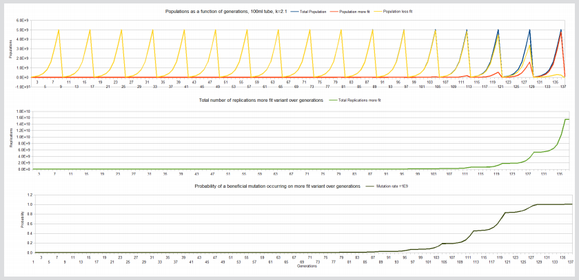
Figure 3: Fixation, total replication more fit variant and probability a beneficial mutation will occur on the more fit variant curves, 100ml tube, k=2.1.
Note: The following curves are for the 100ml tube, k=2.1 experiment
Discussion
Two evolutionary phenomena are occurring in the LTEE. One phenomenon, what Darwin calls the “struggle for existence” or more commonly now called competition which leads to fixation and the other phenomenon is adaptation, the improvement in fitness to an environmental selection condition. The fixation process is a conservative phenomenon. Flake et al. [11] showed that the cost of substitution is associated with a potential energy function and Kimura [12] describes diffusion models to model the changes in gene frequencies in populations over generations. It is well known that diffusion equations are obtained by applying the principles of conservation of energy or mass to control volumes. The carrying capacity of the LTEE is limited by the glucose available in the growth media. That glucose supplies the energy for replication. The competition in the LTEE is for that limited amount of glucose where the more efficient user of that glucose ultimately wins the competition with the less efficient user of glucose.
On the other hand, adaptation is not a conservative phenomenon. Adaptation is a stochastic process where the random trial for improvement in fitness is the replication. There are two possible outcomes for that random trial, a beneficial mutation occurs, or a beneficial mutation does not occur. The frequency for success in this binomial probability problem for a single trial (replication) (Table 3) is the mutation rate times the probability that the particular mutation that occurs is the beneficial mutation. The probability of the adaptation event occurring is dependent on the number of replications of the particular variant that would benefit from that mutation. The more fit variant must amplify (increase in number) in order to improve the probability of the next beneficial mutation occurring on one of the variants. The competition process limits the number of replications of all variants as they compete for the limited resources of the environment. This slows the amplification of the more fit variant. The lower the carrying capacity of the environment, the slower the evolutionary adaptation process is. Fixation in the lower carrying capacity environment occurs more rapidly but adaptation will take more generations of replications as the more fit variant must accumulate the replications necessary for the improvement in the probability of the beneficial mutation occurring. If the mutation rate is 1E-9, from the mathematics of the binomial probability distribution, it will take about a billion replications to get one beneficial mutation on average (Table 4). The more fit variant must first drive the less fit variant to extinction so that all the available resources in the environment are available solely to the more fit variant to achieve the billion replications in a limited carrying capacity environment. The adaptation process will occur most rapidly in a very large carrying capacity environment. Under these conditions, all viable variants can replicate more rapidly by the essentially unlimited resources available in this large carrying capacity environment. This is demonstrated empirically by Baym, et al . [13] and their co-investigators in their mega-plate experiment [13]. An interesting video of this experiment can be found at the following link [14].
The Kishony mega-plate experiment demonstrates that adaptation can occur without fixation occurring. The large petri dish allows sufficient carrying capacity for the drug-sensitive variants to survive as the drug-resistant variants are evolving. The evolving lineages are able to accumulate sufficient replications at each evolutionary step without having to drive the less fit variants to extinction. If a variant can achieve a billion replications, there is a reasonable probability that a beneficial mutation will occur on one of the members of that variant regardless if fixation has occurred or not. The contrast between the LTEE and the Kishony mega-plate experiment demonstrates the difference between competition and adaptation. The three sets of graphs in the illustrations demonstrate how competition affects adaptation for the LTEE. The 10ml, k=1.894 experiment achieves fixation at about 500 generations while at the same time, the more fit variant has achieved the number of replications necessary (4E9) to give a probability very close to 1 that a beneficial mutation will have occurred on the more fit variant.
On the other hand the 1ml, k=2.1 experiment achieves fixation at about 100 generations but has only achieved about 8E7 replications of the more fit variant giving a probability of only about 0.008 that a beneficial mutation has occurred on one of the more fit members. It would take about another 20 days of replications (approximately 120-140 generations) at 5E7 replications per day to give the necessary billion replication and a probability close to 1 of a beneficial mutation occurring on one of its members in that limited carrying capacity environment. And for the 100ml, k=2.1 experiment, it takes 137 generations for fixation but even at generation 127, sufficient replications of the more fit variant have occurred (3E9) for the probability of a beneficial mutation occurring close to 1.
Conclusion
Evolutionary adaptation is mathematically constrained by the mutation rate and the environment carrying capacity. The mutation rate determines how many replications are necessary for a beneficial mutation to occur. The environment carrying capacity determines how quickly these replications can accumulate. It doesn’t matter whether these replications are carried out in a large carrying capacity environment where the replications of other variants do not interfere with replication of the variant that would benefit from the particular mutation or in a limited carrying capacity environment where different variants are competing for a limited amount of resources limiting the growth of all variants.
The variant must be able to attain 1/mutation rate replications to have a reasonable probability of getting on average that beneficial mutation (in a single selection pressure environment). When Haldane wrote [2]: “The principle unit process in evolution is the substitution of one gene for another at the same locus.”, Haldane did not make the distinction between competition and adaptation. Haldane did not have available to him the LTEE and Kishon mega-plate experiment to compare his mathematical model. It is important to understand this difference in understanding evolutionary processes in medicine and agriculture. The carrying capacity of a patient with an infection or cancer is huge, much larger than the carrying capacity of the LTEE. Models of fixation are not adequate to understand these evolutionary processes. It requires adaptation models to correctly explain these evolutionary processes. The failure to understand the difference between competition and adaptation in evolutionary processes is a major cause for misunderstanding how drug-resistance occurs and why cancer treatments fail.
References
- Darwin C (2001) On the Origin of Species. A Penn State Electronic Classics Seriespublication, Copyright © 2001 The Pennsylvania State University. USA
- Haldane JBS (1957) The Cost of Natural Selection. Journal of Genetics, Blackwell Publishing, New York, London, Sydney, Toronto, 55: 511-524.
- Kimura M (1962) On the probability of fixation of mutant genes in a population. Genetics 47(6): 713- 719.
- Hoyle F (1987) Mathematics of Evolution. University College Cardiff Press.
- Schuster P (2011) The Mathematics of Darwin’s Theory of Evolution: 1859 and 150 Years Later.
- Chalub F, Rodrigues J (2011) The Mathematics of Darwin’s Legacy. Mathematics and Biosciences in Interaction. Springer, Basel.
- Benjamin H Good, Igor M Rouzine, Daniel J Balick, Oskar Hallatschek, Michael M Desai et al. (2012) Distribution of fixed beneficial mutations and the rate of adaptation in asexual populations. PNAS 109(13): 4950-4955.
- DM25 Liquid Medium. Richard Lenski Experimental Evolution.
- Kreyszig E (1972) Advanced Engineering Mathematics (3rd ). John Wiley and Sons Inc, New York, London, Sydney, Toronto,
- Kleinman A (2014) The basic science and mathematics of random mutation and natural selection. Statistics in Medicine 33(29): 5074-5080.
- Flake RH, Grant V (1974) An analysis of the cost-of-selection concept. Proc Natl Acad Sci USA 71(9): 3716-3720.
- Kimura M (1964) Diffusion Models in Population Genetics. Journal of Applied Probability 1(2): 177-232.
- Baym M, Lieberman TD, Kelsic ED, Chait R, Gross R, et al. (2016) Spatiotemporal microbial evolution on antibiotic landscapes. Science 353(6304): 1147-1151.
- https://www.youtube.com/watch?v=Irnc6w_Gsas&t=74s
