 Research Article
Abstract
Thermal comfort and sensation are important aspects of the building design and indoor climate control as modern man spends most of the day indoors. Conventional indoor climate design and control approaches are based on static thermal comfort/sensation models that views the building occupants as passive recipients of their thermal environment. Assuming that people have relatively constant range of biological comfort requirements, and that the indoor environmental variables should be controlled to conform to that constant range. Recent advances in mobile technologies in healthcare, in particular wearable technologies (m-health) and smart clothing, have positively contributed to new possibilities in controlling and monitoring health conditions and human wellbeing in daily life applications. The wearable sensing technologies and their generated streaming data are providing a unique opportunity to understand the user’s behaviour and to predict future needs. Many advanced and accurate mechanistic thermoregulation models, such as the ‘Fiala thermal Physiology and Comfort’ model, are developed to assess the thermal strains and comfort status of humans.
However, the most reliable mechanistic models are too complex to be implemented in realtime for monitoring and control applications. Additionally, such models are using not-easily or invasively measured variables (e.g., core temperatures and metabolic rate), which are often not practical and undesirable measurements for monitoring during varied activities over prolonged periods. The main goal of this paper is to develop dynamic model-based monitoring system of the occupant’s thermal state and their thermoregulation responses under two different activity levels. In total, 25 test subjects were subjected to three different environmental temperatures, namely 5° C (cold), 20° C (moderate) and 37° C (hot) at two different activity levels (at rest and cycling). Metabolic rate, heart rate, average skin temperature, skin heat flux and aural temperature are measured continuously during the course of the experiments. The results have shown that a reduced-ordered (second order)s MISO-DTF including three input variables (wearables), namely, aural temperature, heart rate, and average skin heat flux, is best to estimate the individual’s metabolic rate (non-wearable) with mean-absolute-percentageerror of 8.7%.
A general classification model based on least-squares-support-vector-machine (LSSVM) technique is developed to predict the individual’s thermal sensation. For a 7-classes classification problem, the results have shown that the overall model accuracy of the developed classifier is 76% with a F1-score value of 84%.The developed thermal-state prediction model is promising to estimate the human’s thermal sensation/comfort status in real-time and yet reduced-order, which is suitable for wearable applications.
Keywords: Thermal Sensation; Thermal Comfort; Machine Learning; Prediction; Adaptive Controlling
Introduction
Thermal comfort (TC) is an ergonomic aspect determining the satisfaction about the surrounding environment and is defined as ‘that condition of mind which expresses satisfaction with the thermal environment and is assessed by subjective evaluation’ ASHRAE [1]. The effect of thermal environments on occupants might also be assessed in terms of thermal sensation (TS), which can be defined as ‘a conscious feeling commonly graded into the categories cold, cool, slightly cool, neutral, slightly warm, warm, and hot’ ASHRAE [1]. Thermal sensation and thermal comfort are both subjective judgements, however, thermal sensation is related to the perception of one’s thermal state, and thermal comfort to the evaluation of this perception ISO-10551 [2]. The assessment of thermal sensation has been regarded as more reliable and as such is often used to estimate thermal comfort Koelblen et al. [3]. Human thermal sensation is mainly depending on the human body temperature (core body temperature), which is a function of sets of comfort factors Enescu et al. [4,5].
These comfort factors are including indoor environmental factors, namely mean air temperature around the body, relative air velocity around the body, humidity, and mean radiant temperature to the body Parsons [5]. Additionally, some personal (individualrelated) factors, namely, metabolic rate or internal heat production in the body, which vary with the activity level and clothing thermos-physical properties (such as clothing insulation and vapour clothing resistance), are included. It should be mentioned that the individual thermal perception is deepening, as well, on psychological factors include naturalness (an environment where the people tolerate wide changes of the physical environment), expectations and short/long-term experience, which directly affect individuals’ perceptions, time of exposure, perceived control, and environmental stimulation Nikolopoulou et al. [6].
The most considered way to have an accurate assessment of TS is to ask the individuals directly about their thermal sensation perception Enescu et al. [4,5]. Thermal sensation mathematical models have been developed in order to overcome the difficulties of direct enquiry of subjects. The development of such models is mostly depending on statistical approaches that by correlating experimental conditions (i.e., environmental and person-related variables) data to thermal sensation votes obtained from human subjects Koelblen et al. [3,5]. Most of these models (e.g., PMV) are static in the sense that they predict the average vote of a large group of people based on the seven-point thermal sensation scale, instead of individual thermal comfort, they only describes the overall thermal sensation of multiple occupants in a shared thermal environment. To overcome the disadvantages of static models, adaptive thermal comfort models aims to provide insights in increasing opportunities for personal and responsive control, thermal comfort enhancement, energy consumption reduction and climatically responsive and environmentally responsible building design De Dear et al. [7,8].
The idea behind adaptive model is that occupants and individuals are no longer regarded as passive recipients of the thermal environment but rather, play an active role in creating their own thermal preferences De Dear et al. [7]. Besides regression analysis, thermal sensation prediction can also be seen as a classification problem where various classification algorithms can be implemented Lu et al. [8]. Recently, number of research work (e.g., Chaudhuri et al. [9]; Dai et al. [10]; Farhan et al. [11]; Huang, Yang, and Newman [12]; Kim et al. [13] have demonstrated the possibility of using machine learning techniques, such as support vector machine (SVM), to assess and predict human thermal sensation. It can be concluded based on the published work (see the recent literature review by Lu et al. [8] that classificationbased models have performed so well as regression models. Recent advances in mobile technologies in healthcare, in particular wearable technologies (m-health) and smart clothing, have positively contributed to new possibilities in controlling and monitoring health conditions and human wellbeing in daily life applications.
The wearable sensing technologies and their generated streaming data are providing a unique opportunity to understand the user’s behavior and to predict future needs Hussain, Kang, and Lee [14]. The generated streaming data is unique due to the personal nature of the wearable devices. However, the generated streaming data is forming a challenge related to the need of personalized adaptive models that can handle newly arrived personal data. Current HVAC control systems can be divided into two types: air temperature regulator (ATR) and thermal comfort regulator (TCR). Most TCR controllers use static models, mainly PMV, as a performance criterion. This paper is aiming to develop an adaptive model for real-time monitoring of human thermal states using personal non-intrusive sensing techniques. The developed model should be suitable for real-time adaptive controlling of indoor climate systems and smart wearable applications.
Materials and Methods
Experiments and Experimental Setup
Climate Chambers (Body & Mind Room): The “Body & Mind Room” is consisting of three climate-controlled chambers (A, B and C) designed and built to investigate the dynamic mental and physiological responses of humans to specific indoor climate conditions. The Body & Mind Rooms are experimental facilities at the M3-BIORES laboratory (Animal and Human Health Engineering Division, KU Leuven). The three rooms are dimensionally identical; however, each room is designed to provide different ranges of climate conditions as shown in (Table 1).

Table 1: The different temperature and relative humidity ranges that can be provided by the different Body & Mind (A, B and C).
Experimental Protocol: The experimental protocol used in the present study is designed in such way to investigate the subjects’ thermal and physiological responses to predefined three different temperature (low, normal and high) that under two levels of physical activities (seated = low and cycling = high). The three predefined temperatures (low = 5°C, normal = 24°C and high = 37°C) are chosen based on the thermal-comfort-chart of the ASHRAE [15] the effects on health according to the Wind Chill Chart for cold exposure (National Weather Service of the US) and for hot temperatures exposure according to Dewhirst et al. [16]. The conducted experiments are consisted of two phases (Figure 1), upper graph), namely, low activity and high activity phases. During the first experimental phase, low activity phase, the test subjects (while being seated = low activity) are exposed, during 55 minutes, to three levels of temperatures in the following order: normal, low, high and normal again (Figure 1). During the high activity phase, the test subjects is exposed to 15 minutes of light physical stress (80W of cycling on a fastened racing bicycle). During the course (75 minutes) of the active phase, each test subject is exposed to the predefined three temperature levels (Figure 1), lower graph). During each temperature level, starting from the normal level (24 °C), the test subjects are performed 15 minutes of cycling (with 80 W power) and followed 4 minutes of resting (seated). During the course of conducted experiments, the clothing insulation factor (Col) is kept constant at Col = 0.34 which accounts for a cotton short and t-shirt as a standard clothing for all test subjects. The experimental protocol is approved| by the SMEC (SociaalMaatschappelijke Ethische Comissie), on the 16th of January with number G-2018 12 1464.

Figure 1: Plots showing the climate chambers’ set-point temperatures programed during the 55 minutes low activity phase (upper graph) and the 75 minutes high activity phase (lower graph).
Test Subjects: In total 25 healthy participants (6 females and 19 males), between the age of 25 and 35 (average age 26 ± 4.2) years, with average weight and height of 70.90 (±12.70) kg and 1.74 (±0.10) m, respectively, are volunteered to perform the aforementioned experimental protocol.
Measurements and Gold Standards: During the course of the experiments, participants’ heart rate, metabolic rate, average skin temperature, heat flux between the skin and the ambient air, core body temperature represented by the aural temperature are measured continuously. The heart rate monitoring is performed using the Polar H7 ECG strap that is placed under the chest, with a sampling frequency of 128 Hz. The metabolic rate as metabolic equivalent tasks (METs) of each test subject is calculated based on indirect calorimetry using MetaMAX 3B spiroergometer sensor. The average skin temperature is calculated based on measurements from three body-placed, namely, scapula, chest and arm (Figure 2). The skin temperature measurements are performed using one Shimmer temperature sensor and two gSKIN ® bodyTEMP patches. Two heat flux gSKIN ® patches are placed on both the chest and the left arm (Figure 2). The skin temperatures and heat flux measurements are acquired at sampling frequency of 1 Hz. Core body temperature is estimated based on aural temperature measure measurements, which is performed using in-ear wireless (Bluetooth) temperature sensor (Cosinuss One) with a sampling rate if 1Hz. At the end of each applied temperature level during the course of both experimental phases, a thermal sensation questionnaire, based on ASHRAE 7-poins thermal scale, is performed for each test subject.

Figure 2: Sensor placement.
a) Ear channel for aural temperature measurement via the Cosinuss One,
b) Upper arm where skin temperature and heat flux are measured with the gSKIN patch,
c) Middle upper chest where skin temperature and heat flux are measured with the gSKIN patch,
d) Lower chest where heart rate is measured with the Polar H7,
e) Scapula where skin temperature is measured with the shimmer,
f) Mouth and nose where metabolic rate is measured via the MetaMAX-3B spiroergometer sensor.
Modelling and Classification
For the sake of present study, the measured variables are
divided into wearables, which are easily measured variables
using wearable sensors and gold standards (reference) variables,
which are not suitable for wearable technologies. The wearables
are including heart rate  , aural temperature
  , average skin
temperature
, average skin
temperature  , skin heat flux
  and ambient air temperature
 . On the other hand, the gold standards are consisting of the
core temperature
. On the other hand, the gold standards are consisting of the
core temperature  , which is driven from the aural temperature
 , metabolic rate
  and personal thermal sensation
votes TS. The ultimate goal of this work is to develop an adaptive
classification model to predict the individual thermal sensation
depending, solely, on the wearables or estimated variables. Hence,
both of the metabolic rate and core body temperature are estimated
using online dynamic modelling approach (Figure 3). Then, the
individual thermal sensation is predicted using a classification
model (classifier) whose inputs are the wearables and estimated
the metabolic rate and core body temperature (Figure 3).
and personal thermal sensation
votes TS. The ultimate goal of this work is to develop an adaptive
classification model to predict the individual thermal sensation
depending, solely, on the wearables or estimated variables. Hence,
both of the metabolic rate and core body temperature are estimated
using online dynamic modelling approach (Figure 3). Then, the
individual thermal sensation is predicted using a classification
model (classifier) whose inputs are the wearables and estimated
the metabolic rate and core body temperature (Figure 3).
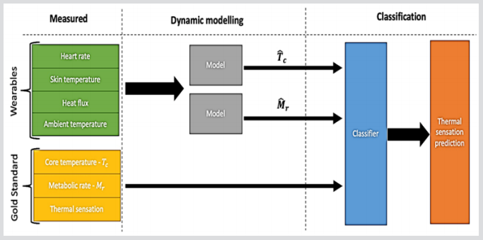
Figure 3: Overview of the main steps to predict the individual thermal sensation.
Dynamic Modelling: Although the system under study (occupant’s thermoregulation) is inherently a non-linear system, the essential perturbation behaviour can often be approximated well by simple linearized Transfer Function (TF) models Young [17,18]. For the purposes of the present paper, therefore, the following liner, Multi-input, single-output (MISO) discrete-timesystems are considered to estimate metabolic rate and core body temperature Young [19] ,
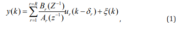
where denotes the value of the asscociated variable at the th
sampling instant; is the output variable;  are input variables,
while
are input variables,
while  and
and  are appropriately defined polynomials in
the backshift operator
are appropriately defined polynomials in
the backshift operator  , i.e.,
 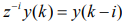 and
and  is
additive noise, a serially uncorrelated sequence of random variables
with variancethat accounts for measurement noise. The Simplified
Refined Instrumental Variable (SRIV) algorithm was utilised in the
identification and estimation of the models (model parameters and
model structure) Young and Jakeman [20]. Two main statistical
measures were employed to determine the most appropriate model
structure. Namely, the coefficient of determination , based on the
response error; and YIC (Young’s Information Criterion), which
provides a combined measure of model fit and parametric efficiency,
with large negative values indicating a model which explains the
output data well and yet avoids over-parameterisation Young,
Chotai and Tych [21] . Additionally, the estimation performance
of the selected models is evaluated used the mean-absolute-error
(MAE) value.
is
additive noise, a serially uncorrelated sequence of random variables
with variancethat accounts for measurement noise. The Simplified
Refined Instrumental Variable (SRIV) algorithm was utilised in the
identification and estimation of the models (model parameters and
model structure) Young and Jakeman [20]. Two main statistical
measures were employed to determine the most appropriate model
structure. Namely, the coefficient of determination , based on the
response error; and YIC (Young’s Information Criterion), which
provides a combined measure of model fit and parametric efficiency,
with large negative values indicating a model which explains the
output data well and yet avoids over-parameterisation Young,
Chotai and Tych [21] . Additionally, the estimation performance
of the selected models is evaluated used the mean-absolute-error
(MAE) value.
Classification Model: To predict the individual thermal
sensation, a classification model (classifier) is developed and trained
based on the wearables and estimated variables (metabolic rate and
core body temperature) that together with the thermals sensation
votes (gold standard). A modified support vector machine (SVM)
technique, namely, least-squares support vector machine (LS-SVM)
is used to develop and train the thermal sensation classifier Suykens
et al. [22]; Suykens and Vandewalle [23]. SVMs are originally
presented as binary classifiers Suykens et al. [22] that assign each
data instance  to one of two classes described by a class
label
to one of two classes described by a class
label  based on the decision boundary that maximises the
margin
based on the decision boundary that maximises the
margin  between the two classes. Generally, a feature map
 is used to transform the geometric boundary
between the two classes to a linear boundary
is used to transform the geometric boundary
between the two classes to a linear boundary  in
feature space, for some weight vector
in
feature space, for some weight vector  and
and  . The
class of each instance can then be found by
. The
class of each instance can then be found by 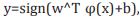 where sign refers to the sign function.
Due to some computational complexities of standard SVM because of the quadratic programming problem, least squares support vector machines (LS-SVM) is presented to overcome such problem. LS-SVM, in contrast with standard SVM, relies on least squares cost function as follows:

such that; 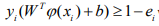 where
where  errors such that
 is proportional to the signed distance of x_i from the decision
boundary, and
is proportional to the signed distance of x_i from the decision
boundary, and  represents the regularisation constant. In LSSVM, instead of solving the quadratic programming problem a set
of linear equations to be solved is sufficient to find the optimal
solution of the classifier. The LS-SVMlab (Least Squares Support
Vector Machine lab) Matlab-based toolbox is used to implement the
LS-SVM classification algorithm Suykens et al. [22].
represents the regularisation constant. In LSSVM, instead of solving the quadratic programming problem a set
of linear equations to be solved is sufficient to find the optimal
solution of the classifier. The LS-SVMlab (Least Squares Support
Vector Machine lab) Matlab-based toolbox is used to implement the
LS-SVM classification algorithm Suykens et al. [22].
The performance of the classification model is determined based on accuracy, sensitivity, precision and F1-score as follows:
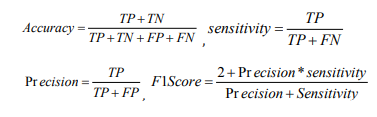
where TP, TN, FP and FN are the true positive, true negative, false positive and false negative, respectively.
Results and Discussion
Dynamic Modelling and Estimation of Individual’s Metabolic Rate
The average metabolic rate obtained from the 25 participants
at the temperature levels (24, 5 and 37 °C) during low and high
activity phases are presented in (Table 2). Different combinations
of inputs variables (wearables) are tested for best estimation
of individual’s metabolic rate. The SRIV algorithm, combined
with and selection criteria, suggested that a second-order MISO
discrete-time TF with heart rate (  ), average skin heat flux (
  ) and aural temperature (
 ) as input variables is the best (with
average = 0.89 ±0.04 and = − 13.62 ±2.33) to describe and estimate
the dynamic behaviour of the individual’s metabolic rate. More
specifically, the SRIV algorithm identified the following general
MISO discrete-time TF model structure
) as input variables is the best (with
average = 0.89 ±0.04 and = − 13.62 ±2.33) to describe and estimate
the dynamic behaviour of the individual’s metabolic rate. More
specifically, the SRIV algorithm identified the following general
MISO discrete-time TF model structure
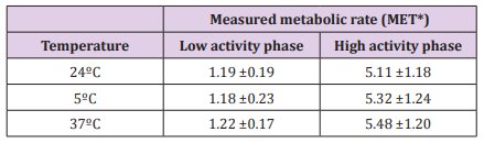
Table 2: Average (±standard deviation) of the measured metabolic rate obtained from the 25 test subjects during low and high activity phases.
Note: 1MET = 1.163 W.kg-1
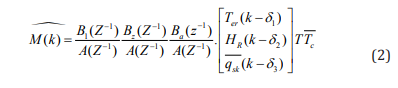
where  is the estimated metabolic rate and the numerator
polynomials , and are of the following orders (number of zeros)
2, 3 and 2, respectively. While the system delays , and are varied
from person to another (inter-personal) with average values of
1.4, 0.20 and 0.21 minutes, respectively. A simulation example of
the developed estimation model (2) for one test subject during low
activity experimental phase at normal temperature (24°C) depicted
in (Figure 4).
is the estimated metabolic rate and the numerator
polynomials , and are of the following orders (number of zeros)
2, 3 and 2, respectively. While the system delays , and are varied
from person to another (inter-personal) with average values of
1.4, 0.20 and 0.21 minutes, respectively. A simulation example of
the developed estimation model (2) for one test subject during low
activity experimental phase at normal temperature (24°C) depicted
in (Figure 4).

Figure 4: A simulation example of the developed MISO-DTF model (2) to estimate the metabolic rate during the low activity experimental phase at normal temperature (24oC).
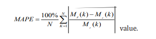
The estimation performance of the selected general MISO-DTF (2) is evaluated based on the mean-absolute-percentage-error
The results have shown that the developed general model is shown, for all test subjects, a higher average MAPE value (10 ±2.2 %) during the low activity phases than the average MAPE value (7.6 ±2.6 %) resulted during the high activity phases. The METs (metabolic equivalent tasks) are a measure, which accounts for a normalized form of energy expenditure per kilogram of mass. There are consensus that the measurement of metabolic rate might vary amongindividuals (interpersonal) up to 75% Byrne et al. [24] and even within the same day from morning to afternoon for the same subject (intrapersonal) up to 6%, though measurements on different days might be comparable on fasted subjects Haugen et al. [25] . Hence, a general estimation model of individual metabolic rate will not be efficient in this case. However, the general estimation performance of the suggested general MISO model can be enhanced by using the online adaptive form of the SRIV algorithm Garnier, Young and Gilson [26]. The online adaptive (closed-loop) SRIV algorithm is providing the possibility to personalise the developed general model by retuning the model parameters and model delays based on the streaming data acquired from the wearable sensors (Table 3).
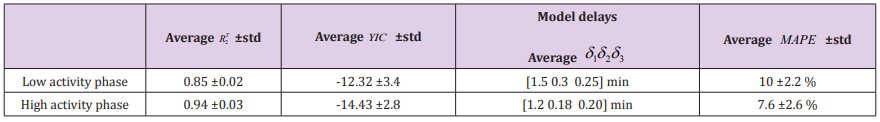
Table 3: Average RT2, YIC model delays and MAPE for the selected MISO-DTF model to estimate the individual’s metabolic rate obtained from the 25 test subjects during low and high activity phases.
Classification Model and Prediction of Individual’s Thermal Sensation
In order to give an idea about the interaction relationship
between considered variables, the correlation between all
measured variables are calculated and represented in a colourmap correlation coefficient (r) matrix as shown in (Figure 5).
High positive or negative correlation coefficient values, such as
that between heat flux and skin temperature, are reflected strong interaction between these variables, which can affect the feature
selection of the classification model. The classification model for
predicting the individual’s thermal sensation is developed, based
on LS-SVM approach, by training the classifier on 80% of the data
points, while the rest of the data (20%) is used for testing. The
model accuracy, sensitivity F1-score and overall confusion matrix
are computed to evaluate the performance of the developed
classifier. A feature space including all the measured and estimated
input variables, namely,  and
and  . Additionally, other features are extracted by computing the
variance, min, max, root mean squares (RMS) and first derivative
(
. Additionally, other features are extracted by computing the
variance, min, max, root mean squares (RMS) and first derivative
( where is the variable) of the aforementioned measured and
estimated variables. The age and gender of the test subjects are also
included in the feature spaces.
where is the variable) of the aforementioned measured and
estimated variables. The age and gender of the test subjects are also
included in the feature spaces.
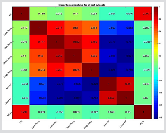
Figure 5: Colour-map of the correlation matrix representing the correlation levels (r∈[-1,1]) between the mean values of all measured variables, namely, heart rate (HR), aural (core) temperature, arm temperature, chest temperature, scapula temperature, heat flux from the arm skin (Arm HF), heat flux from the chest skin (Chest HF) and metabolic rate (MET’s).
(Figure 6) is showing the distribution of the participants’ thermal sensation votes at the three environment temperatures (24, 5 and 37 °C). The aforementioned figure is showing the ‘confusion space’, or the area in which the reported thermal sensation votes at the three environmental temperatures are overlapping. Such observation shows that the thermal perception may overlap even with big difference in the surrounding environmental temperatures. Such confusion space is a great challenge for any predictive model of thermal sensation especially for static models such as PMV. For the sake of the main objective of the present work, the computational cost of the developed algorithm should be low enough to be compatible with wearable technology and online modelling. Hence, a feature selection procedure is employed to obtain the most reduced-dimension model yet with best error performance. Feature selection here is based on evaluating all possible feature combinations and selecting the combination with best error performance. The feature selection step is resulted in a feature space including 25 features as shown in (Table 4).
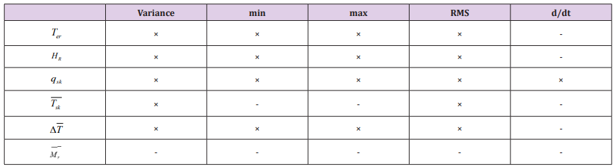
Table 4: An overview of the selected feature space including the measured and estimated variables (six variables) and some operations on these variables (× = selected).
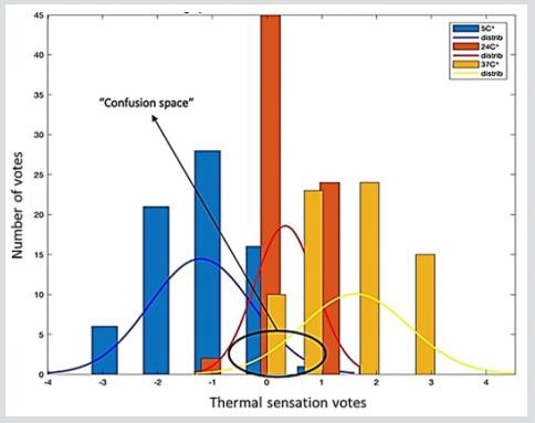
Figure 6: Distribution of the participants (25) thermal sensation votes at the three environment temperatures (24, 5 and 37 °C) showing the confusion space.
A classification model is developed based on the selected 25 input features and trained using the LS-SVM approach. The resulted confusion matrix from the developed classification model based on the selected feature space is shown in (Figure 6) and Figure 7. The overall error performance results of the developed classification model are presented in (Table 4). For a 7-classes classificatison problem, the developed classifier has shown an overall accuracy of 76% to predict the individual’s thermal sensation. The developed classifier has shown a high (84%) F1-score, which reflects low false positive and negative.
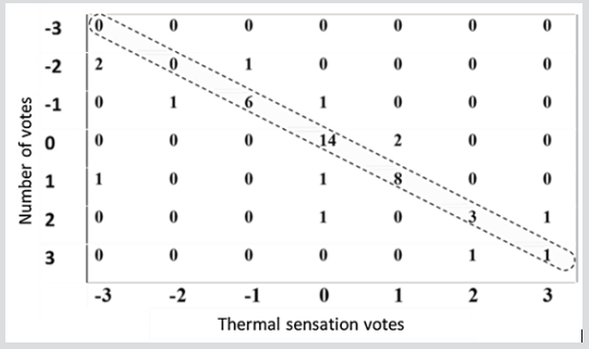
Figure 7: The resulted confusion matrix from testing the developed LS-SVM classifier. The diagonal represents the correctly classified data points.
Table 5 The error performance results of the developed general classification for each class separately are shown in (Table 6). The results showed that the error performances of classes 1, 2, 6 and 7 are very low see (Table 6), which can be attributed to the low number (0, 2, 4, 2, respectively) of obtained votes for these classes or in other word due to the uneven class distribution. Therefore, the overall F1-score is more reliable and efficient measure of performance than accuracy in this case. SVM is used in recent studies to assess occupant’s thermal demands Dai et al. (2017), and to predict thermal comfort/sensation Farhan et al. (2015).
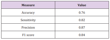
Table 5: Overall error performance (accuracy, sensitivity, precision and F1-score) of the developed general LS-SVM classification model.
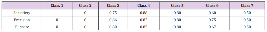
Table 6: The error performance (precision, sensitivity, and F1-score) of the developed general LS-SVM model for the 7-classes classification problem.
In this present paper, 25 participants are subjected to three different environmental temperatures, namely 5°C (cold), 20 °C (moderate) and 37 °C (hot) at two different activity levels, namely, at low level (rest) and high level (cycling at 80 W power). Metabolic rate, heart rate, average skin temperature (from three different body locations), heat flux and aural temperature are measured continuously during the course of the experiments. The thermal sensation votes are collected from each test subject based on ASHRAE 7-points questioner. The results have shown that a reduced-ordered (second order) MISO-DTF including three input variables (wearables), namely, aural temperature, heart rate, and average heat flux, is best to estimate the individual’s metabolic rate (non-wearable) with average MAPE of 8.7%. A general classification model based on LS-SVM technique is developed to predict the individual’s thermal sensation. For a 7-classes classification problem, the results have shown that the overall model accuracy and F1-score of the developed classifier are 76% and 84%, respectively. It is suggested in this paper that the model overall performance of the model can be enhanced by using a personalised adaptive classification algorithm based on streaming data from wearable sensors.
References
- (2004) ASHRAE, Thermal Environmental Conditions for Human Occupancy. ASHRAE Sta. Atlanta GA: American Society of Heating, Refrigeration and Air Conditioning Engineers, Inc.
- (1995) ISO-10551. Ergonomics of the Thermal Environment -Assessment of the Influence of the Thermal Environment Using Subjective Judgement Scales. Brussels.
- Koelblen B, A Psikuta, A Bogdan, S Annaheim, RM Rossi (2017) Thermal Sensation Models: A Systematic Comparison. Indoor Air 27(3): 680-689.
- Enescu Diana (2019) Models and Indicators to Assess Thermal Sensation Under Steady-State and Transient Conditions. Energies 12(5): 841.
- Parsons KC (2014) Human Thermal Environments: The Effects of Hot, Moderate, and Cold Environments on Human Health, Comfort, and Performance, (3rd ). CRC Press.
- Nikolopoulou Marialena, Koen Steemers (2003) Thermal Comfort and Psychological Adaptation as a Guide for Designing Urban Spaces. Energy and Buildings 35(1): 95-101.
- De Dear, Richard, Gail Schiller Brager (1998) Developing an Adaptive Model of Thermal Comfort and Preference. ASHRAE Transactions 104(1): 145-167.
- Lu Siliang, Weilong Wang, Shihan Wang, Erica Cochran Hameen, Siliang Lu, et al. (2019) Thermal Comfort-Based Personalized Models with Non-Intrusive Sensing Technique in Office Buildings. Applied Sciences 9(9): 1768.
- Chaudhuri Tanaya, Yeng Chai Soh, Hua Li, Lihua Xie (2017) Machine Learning Based Prediction of Thermal Comfort in Buildings of Equatorial Singapore. In 2017 IEEE International Conference on Smart Grid and Smart Cities (ICSGSC), IEEE p. 72-77.
- Dai Changzhi, Hui Zhang, Edward Arens, Zhiwei Lian (2017) Machine Learning Approaches to Predict Thermal Demands Using Skin Temperatures: Steady-State Conditions. Building and Environment 114: 1-10.
- Farhan Asma Ahmad, Krishna Pattipati, Bing Wang, Peter Luh (2015) Predicting Individual Thermal Comfort Using Machine Learning Algorithms. In 2015 IEEE International Conference on Automation Science and Engineering (CASE), IEEE pp. 708-713.
- Huang Chuan Che, Rayoung Yang, Mark W Newman (2015) The Potential and Challenges of Inferring Thermal Comfort at Home Using Commodity Sensors. In Proceedings of the 2015 ACM International Joint Conference on Pervasive and Ubiquitous Computing, New York, USA, pp. 1089-1100.
- Kim Joyce, Yuxun Zhou, Stefano Schiavon, Paul Raftery, Gail Brager (2018) Personal Comfort Models: Predicting Individuals thermal Preference using Occupant Heating and Cooling Behavior and Machine Learning. Building and Environment 129: 96-106.
- Hussain Shujaat, Byeong Ho Kang, Sungyoung Lee (2014) A Wearable Device-Based Personalized Big Data Analysis Model. In Lecture Notes in Computer Science, Springer, Cham pp. 236-242.
- (2017) ASHRAE ASHRAE Standard 55. Atlanta GA: American Society of Heating, Refrigerating and Air-Conditioning Engineers, INc.
- Dewhirst MW, BL Viglianti, M Lora Michiels, M Hanson, PJ Hoopes (2003) Basic Principles of Thermal Dosimetry and Thermal Thresholds for Tissue Damage from Hyperthermia. International Journal of Hyperthermia 19(3): 267-294.
- Young Peter C (1989) Advances in Theory and Applications. (Eds.), CT Leondes, Control and Dynamic Systems Elsevier p. 1-427.
- Youssef Ali, Maarten D Haene, Jochen Vleugels, Guido De Bruyne, Jean Marie Aerts (2018) Localised Model-Based Active Controlling of Blood Flow During Chemotherapy to Prevent Nail Toxicity and Onycholysis. Journal of Medical and Biological Engineering 39(4): 1-12.
- Young Peter C (1993) Concise Encyclopedia of Environmental Systems. first. PERGAMON-ELSEVIER SCIENCE LTD.
- Young Peter C, Anthony Jakeman (1980) Refined Instrumental Variable Methods of Recursive Time-Series Analysis Part III. Extensions. International Journal of Control 31(4): 741-764.
- Young Peter C, Arun Chotai, Wlodek Tych (1991) Identification, Estimation and Control of Continuous-Time Systems Described by Delta Operator Models. Identification of Continuous Time Systems pp. 363-418.
- Suykens Johan AK, Tony Van Gestel, Jos De Brabanter, Bart De Moor, Joos Vandewalle (2002) Least Squares Support Vector Machines. World Scientific pp. 308.
- Suykens JAK, J Vandewalle (1999) Least Squares Support Vector Machine Classifiers. Neural Processing Letters 9(3): 293-300.
- Byrne Nuala M, Andrew P Hills, Gary R Hunter, Roland L Weinsier, Yves Schutz (2005) Metabolic Equivalent: One Size Does Not Fit All. Journal of Applied Physiology 99(3): 1112-1119.
- Haugen Heather A, Edward L Melanson, Zung Vu Tran, Jay T Kearney, James O Hill (2003) Variability of Measured Resting Metabolic Rate. American Journal of Clinical Nutrition 78(6): 1141-1145.
- Garnier Hugues, Peter C Young, Marion Gilson (2009) Simple Refined IV Methods of Closed-Loop System Identification. IFAC Proceedings 42(10): 1151-1156.
