The Estimation of the Instantaneous Amplitudes and the Instantaneous Frequencies of the EEG when both are Stochastic Process Volume 48- Issue 2

Ahmed S Abutaleb¹* and H Soliman²

• ¹Previously with MIT Lincoln Lab, Lexington, MA, USA. And currently with Cairo University, School of Engineering, Systems and Bioengineering Departments. Giza, Egypt
• ²School of Medicine, Beny Swaif University, Egypt

Received:December 21, 2022;   Published:January 24, 2023

*Corresponding author: Ahmed S Abutaleb, Previously with MIT Lincoln Lab, Lexington, MA, USA. And currently with Cairo University, School of Engineering, Systems and Bioengineering Departments. Giza, Egypt

DOI: 10.26717/BJSTR.2023.48.007621

Abstract PDF

In this report we model the EEG signal as a sum of sine waves. Each sine wave has a random frequency and a random amplitude. We use band pass filters to separate the different frequency segments of the EEG. The frequency is modeled as an Ornstein- Uhlenbeck (OU) stochastic process i.e., the frequency is bouncing around a mean value. In each EEG band, an adaptive filter is developed to estimate the random frequency. The instantaneous amplitude is then obtained by using adaptive noise cancelling where one channel is the EEG band pass signal and the other channel is the estimated sine wave with random frequency. Another amplitude estimate is obtained by using an energy separation operator with the estimated frequency. The results are compared to the Teager energy separation operator (TEO) and showed better performance

Keywords: EEG; Sotchastic Differential Equation; Adaptive Filter; Adaptive Noise Cancelling; Teager Energy Operator

Abbreviations: OU: Ornstein-Uhlenbeck; TEO: Teager Energy Separation Operator; EMD: Empirical Mode Decomposition; HHT: Hilbert-Huang Transform; FT: Fourier Transform; DESA: Discrete Energy Separation Algorithm; RLS: Recursive Least Square

The modulated sine wave is a common model for signals used in communications, speech analysis, and EEG analysis IEEE [1] Van Zaen [2] among others. The modulation could be in the amplitude, the frequency, or both. The estimation of the modulated signal parameters is known in the literature as the AM-FM signal problem. The objectives are to estimate the instantaneous amplitude and the instantaneous frequency. Due to the considerable non-stationary and nonlinear characteristics of the EEG, commonly used methods based on Fourier transform (FT) provide the resulting frequency spectrum with only little physical sense. Therefore, several methods to analyze spectrum of such signals have been developed in past decades. Hilbert-Huang Transform (HHT) is one of these methods. HHT is based on empirical mode decomposition (EMD), followed by Hilbert transform to compute Hilbert spectrum [Huang, et al. [3]]. Teager energy operator (TEO) which is a discrete energy separation algorithm (DESA) [Maragos, et al. [4,5]] is commonly used for the estimation of the instantaneous amplitude and the instantaneous frequency. Unfortunately, the accuracy of the TEO deteriorates rapidly as the signal to noise ratio of the observations gets lower or as the fluctuations in the amplitude or frequency are relatively high. Nevertheless, it was used in several EEG analysis studies [Kamath [6]].

In many situations the observed signal is modeled as a sum of sinusoids with random amplitude [Wehner [7]] [Li; 1998]. The randomness could be imbedded in the additive noise term or could be modeled by itself. The random amplitude situation occurs for example with fading channels, fluctuating targets [Van Trees [8]], random media … etc [Barkat [9]]. In this report, the focus is on the estimation of the instantaneous amplitude and the instantaneous frequency of the EEG bands. The random frequency could be modeled as an AR process, MA process, or a polynomial [Benidir, et al. [10,11]]. The coefficients of the model are estimated adaptively using the least mean square algorithm (LMS), the recursive least square (RLS) algorithm, or others such as hidden Markov models [IEEE [1,12]]. Other methods, based on stochastic calculus, were developed to tackle the problem of the estimation of stochastic amplitude and stochastic phase [Abutaleb, et al. [13-15]]. These methods differ in the proposed model for the amplitude and or phase. In this report, the frequency is represented as an Ornstein-Uhlenbeck stochastic process, while the amplitude is time varying but unknown. In Section II, we present the EEG parameter estimation problem and the commonly used TEO. In Section III, we introduce our proposed approach based on adaptive filters and we derive the estimation equations for both the instantaneous amplitude and the frequency. In Section IV, we present simulation and real data results. We also present conclusions and summary.

In this section we present the problem at hand and present the conventional TEO to estimate the instantaneous amplitude and frequency. Considering the multiple characteristic bands of EEG, we can also interpret the EEG as a multicomponent AM-FM signal. An EEG signal can thus be written as a linear combination of amplitude and frequency modulated components.
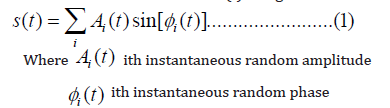
Let the observed EEG be defined as s(t) and given as:

In this report, a band pass filter is used to separate the different EEG bands (delta, theta, alfa, beta, and gamma). Thus, the focus is on one band at a time. The same process could be repeated for other bands.
Let the received real signal, z(t), after band pass filter with random amplitude be modeled as:

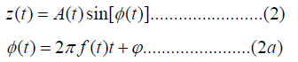
Where f(t) follows an OU process and is the unknown but deterministic constant phase.
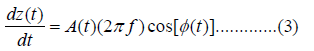
In TEO method, we assume slowly varying amplitude. Taking the first derivative with respect to time of the signal z(t) we get:

Taking the second derivative with respect to time, assuming constant amplitude, we get:

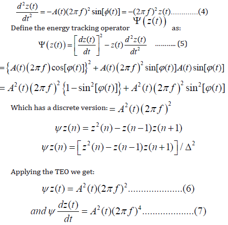
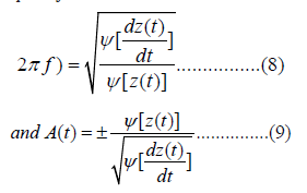
Hence the estimates of the instantaneous amplitude and the instantaneous frequency are obtained as:

In this section we present in some detail the proposed approach to find an estimate of the amplitude and the frequency of the band passed signal. The summary of the steps follows:
1) An OU model is assumed for the frequency while keeping the phase deterministic but unknown,
2) We then develop the adaptive filter to estimate the frequency assuming constant amplitude of unity magnitude,
3) Using the estimated frequency, a sinusoidal wave is generated,
4) This sinusoidal wave with unity amplitude but random frequency is used as a reference signal,
5) An adaptive noise cancelling (ANC) filter, with the estimated sine wave as reference, is used to find an estimate for the time varying amplitude through division or others,
6) We use a hybrid approach where the estimated frequency is substituted in the TEO equations to get an estimate of the instantaneous amplitude,
7) Finally, the estimated amplitude/frequency is compared to the TEO based amplitude/frequency.

The frequency f(t) is modeled as an Ornstein-Uhlenbeck process. The stochastic differential equation (SDE) that describes the frequency is given as [Abutaleb, et al. [16]]:

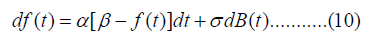
The model expresses a signal that is, randomly, bouncing around a constant value β . The strength of the randomness is controlled by σ . The frequency f(t) might take an excursion away from the mean β . It eventually returns to this meaning. The average length of these excursions is controlled by the parameterα . Other forms of f(t) are also valid and might be useful [Neftci [17]].

A single sine wave, X(t), is modeled as:

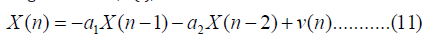
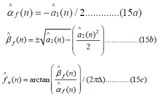
Where v(n) is white Guassian noise with zero mean and unity variance, a₁ and a₂ are unknown quantities that determine the frequency f according to the equation:

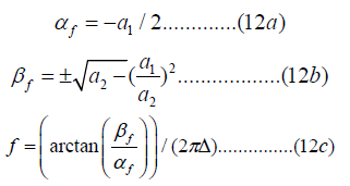
where Δ is the sampling interval. Notice that the arctan operation yields the phase between “ −π ” and “ +π ”. Thus, we have a sine wave X(n) with frequency f. The phase is determined from the initial conditions X(-1) and X(0). To obtain an initial guess for the frequency, we assume that we have a sine wave with unknown frequency and unknown phase. The amplitude is assumed to be of unity magnitude. We use least square between the observed EEG signal and the assumed sine wave, to find an initial guess for the frequency. Thus, initial guesses are obtained for a₁ , a₂ , X(-1) and X(0).

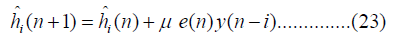
We use the LMS algorithm to find an updated estimate of the frequency. We first estimate the changing coefficients according to the equation:

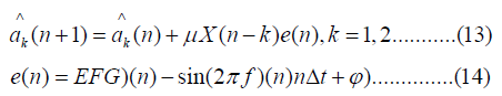
Where EEG(n) is the observed band limited EEG signal, and the estimated frequency is given as:

Once we have estimated the parameters of the OU process describing the amplitude and the parameters of the frequency, we move ahead and find an estimate for the amplitude itself.
Remember that:

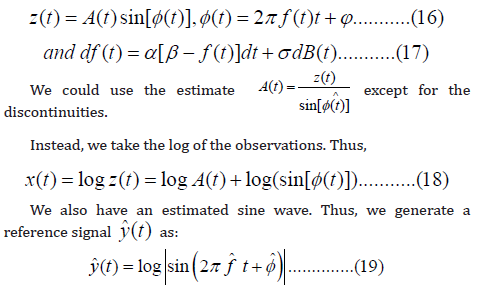
The observed signal (x(t)=log z(t)) is made of two parts: (1) log A(t) and (2) y(t) = log(sin[φ (t)] ). An estimate yˆ(t) of the second part, y(t), is available. In adaptive noise cancelling we pass the estimated signal yˆ(t) through an adaptive filter and subtract from x(t) to find an estimate for log A(t) [Abutaleb, et al. [16]]. Specifically.
Define

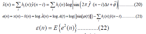
Where Δt is the sampling interval, hi (n) are the adaptive filter coefficients that will be recursively estimated. To find the unknown coefficients, hi (n) , we minimize the sum of squared error w.r.t. the coefficients hi (n) . The adaptive filter weights, hˆ_i (n) , are updated through the least mean square (LMS) algorithm as:

We then take the exponent of the estimated log Aˆ(n) from eqn. (III. 10) to get an estimate for the instantaneous amplitude Aˆ(n) . Unfortunately, this estimate usually has discontinuities. We use a moving average (MA) filter to smooth away these discontinuities. Notice that there is an ambiguity in the sign of the amplitude A(t) unless it is assumed to be positive value. The TEO will be used for comparison with the proposed approach.

Since TEO has good amplitude estimation and bad frequency estimation, one could use the estimated frequency, from the adaptive filter, to get an estimate for the amplitude. Specifically, if we have an estimate fˆ for f(t) (see equation III. 6c) we could use the expression

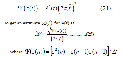
and Δ is the sampling interval. This approach yielded better results even at SNR less than 10 db.

1) Use band pass filter to isolate each frequency component
2) Use the FFT to find initial estimates of frequency and amplitude
3) Use least square to find the estimates of the frequency and phase.
4) Use the adaptive filter to find estimates of the instantaneous frequency.
5) Use adaptive noise cancelling filter to find an estimate of the amplitude.
6) The artificial speckle noise through the moving average (MA) filter.
7) Use the hybrid approach to find an estimate of the amplitude.

In this section we simulate, for different signal to noise ratio, a sine wave with time-varying frequency that follows an OU process. We show the results of the estimation using the steps described in Section III. We also use the TEO operator to find the estimates of the amplitude and the frequency. We then apply the same methods to real EEG data.

Figure 1.

Figure 2.

The sampling interval is taken to be 10 msec, the frequency is 12 Hz., the phase is π / 4 . The frequency f(t) is modeled as an OU process

with coefficients = α =10,β =1andσ = 2
In (Figure 3), we show the simulated frequency using equation.
We use the SNR of the estimate for comparison. The SNR for the estimate is defined as:

Figure 3.

Figure 4.

Figure 5.

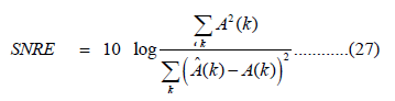
Following the estimation steps of Section III, we present, in (Figure 4), the estimated amplitude using the adaptive noise cancelling filter equations. In (Figure 5), we present the same amplitude after passing through the moving average filter. The SNRE was 11.2 db.

In (Figure 6), we present the estimated amplitude using the TEO. In (Figure 7) we present the amplitude after passing through the MA filter. The SNRE was 8.5 db. We now present the results of real data of EEG. As a demonstration, we use the signal coming from T3-AV. The estimated amplitudes, using TEO and the proposed method, for the bands, delta, alfa, theta, and beta are shown in (Figures 8-11). Notice that the estimated amplitude using the TEO method tends, in most cases, to be larger than that using adaptive noise cancelling.

Figure 6.

Figure 7.

Figure 8.

Figure 9.

Figure 10.

Figure 11.

In summary, the proposed approach has the following advantages over the TEO
1) Better frequency estimation accuracy as shown in simulation.
2) The estimation of the mean reverting value of the amplitude β. This estimate gives an indication of the average value of the amplitude and will tell us whether the instantaneous amplitude estimates are reasonable or not.
3) The estimation of the frequency and the phase. So even if the frequency is slightly changing, this estimate will guide us through the calculations. This is unlike TEO where you are not sure about the real values of the frequencies.
The presented stochastic calculus-based approach could be extended to the case that both the amplitude and phase are randomly changing. This and other issues are currently under investigation [Y Cho, et al. [18]].

1. IEEE Proceedings (1996) Special Issue on Instantaneous Frequency Estimation 84(9).
2. Van Zaen J (2012) Efficient Schemes for Adaptive Frequency Tracking and their Relevance for EEG and ECG, Ph. D. Dissertation, ÉCOLE POLYTECHNIQUE FÉDÉRALE DE AUSANNE, Switzerland.
3. QH Huang, J Yang, Y Zhou (2008) Bayesian nonstationary source separation, Neurocomputing 71: 1714-1729.
4. Maragos P, J Kaiser, T Quatieri (1992) On separating amplitude from frequency modulations using energy operators”, [Proceedings] ICASSP-92: 1992 IEEE International Conference on Acoustics, Speech, and Signal Processing.
5. Pal S, B Biswas (2012) On the Fundamental Aspects of Demodulation. Signal Processing: An International Journal (SPIJ) 6 (3): 86-96.
6. Kamath C (2014) Automatic seizure detection based on Teager Energy Cepstrum and pattern recognition neural networks. QScience Connect 2014 (1).
7. Wehner D (1995) High Resolution Radar, Artech House, Mass, USA. 
8. H Van Trees (1970) Detection, Estimation and Modulation Theory, Part III, John Wiley, NY.
9. Barkat B (2001) Instantaneous Frequency Estimation of Nonlinear Frequency Modulated Signals in the Presence of Multiplicative and Additive Noise.IEEE Trans. Signal Processing 49(10): 2214-2222.
10. M Benidir, A Ouldali (1999) Polynomial Phase Signal Analysis Based on the Polynomial Derivatives Decomposition. IEEE Trans. Signal Processing 47(7): 1954-1965.
11. Goto S, M Nakamura, K Uosaki (1995) Online Spectral Estimation of Nonstationary Time Series Based on AR Model Parameter Estimation and Order Selection with a Forgetting Factor. IEEE Trans. Signal Processing SP-43 (6): 1519-1522.
12. Boashash B (1992) Estimating and Interpreting the Instantaneous Frequency of a signal. Proc IEEE 80(4).
13. Abutaleb A (2013) The estimation of the instantaneous amplitudes of sum of sinusoids with unknown frequencies and phases: The martingale approach”, Signal Processing 93 (4): 811-817.
14. Abutaleb A (2005a) Instantaneous Frequency Estimation When the Amplitude is a Stochastic Process Using Stochastic Calculus and Bootstrapping. Circuits, Systems and Signal processing 24 (1): 35-52.
15. Abutaleb A (2005b) Instantaneous Frequency Estimation Using Stochastic Calculus and Bootstrapping., EURASIP Journal on Applied Signal Processing 12: 1886-1901.
16. Abutaleb A (1988) Improvement in Adaptive Noise Canceling Using a Nonlinear Filter Based On The Pontryagin Minimum Principle. Circuits, Systems and Signal processing 7(1): 57-78.
17. Neftci S (2000) An Introduction to the Mathematics of Financial Derivatives, Academic Press, New York.
18. Y Cho, S Kim, E Powers (1991) Time-Varying Spectral Estimation Using AR Models with Variable Forgetting Factors. IEEE Trans. ASSP 39(6): 1422-1426.