Class Based Variable Importance for Medical Decision Making Volume 1 - Issue 5

Atara Posner¹, Farhad Azimi¹, David Goltsman² and Sanjay Warrier^1,2*

• ¹Chris OBrien Life house Centre, Australia
• ²Institute of Academic Surgery, RPA, Australia

Received: September 29, 2017;   Published: October 12, 2017

Corresponding author: Danielle Baghernejad, Intermedix, Nashville TN 37219, Tennessee, USA

DOI: 10.26717/BJSTR.2017.01.000431

Abstract PDF

In this paper we explore variable importance within tree-based modeling, discussing its strengths and weaknesses with regard to medical inference and action ability. While variable importance is useful in understanding how strongly a variable influences a tree, it does not convey how variables relate to different classes of the target variable. Given that in the medical setting, both prediction and inference are important for successful machine learning, a new measure capturing variable importance with regards to classes is essential. A measure calculated from the paths of training instances through the tree is defined, and initial performance on benchmark datasets is explored.

Keywords : Machine learning; Tree-based modeling; Decision trees; Variable importance; Class Variable Importance

Abbreviations : CART: Classification and Regression Trees; CVI: Class Variable Importance; ET: Extra Trees; RF: Random Forests; GBT: Gradient Boosted Trees; AUC: Area under the Curve; ROC: Receiver Operating Characteristic

Tree based methods are common for use with medical datasets, the goal being to create a predictive model of one variable based on several input variables. The basic algorithm consists of a single tree, whereby the input starts at the root node and follows a path down the tree, choosing a path based on a splitting decision at each interior node [1]. The prediction is made by whatever leaf node the path ends in, either the majority or average of the node, depending on whether the problem is classification or regression respectively. Several implementations exist, such as ID3 [1,2], C4.5 [1,3] and CART (Classification and Regression Trees) [2], with CART being the implementation in Python’s scikit-learn machine learning library used in this analysis. More sophisticated algorithms build on the simple tree by making an ensemble of thousands trees, pooling the predictions together for a single final prediction. Prominent among these are Random Forests [3], Extra Trees [4-9], and Gradient Boosted Trees [6].

Tree based modeling in itself is popular given that it is easy to use, can easily support multi class prediction, and is better equipped to deal with small n and large p problems, where the number of observations are much smaller than the number of variables. The small n, large p issue is especially relevant in certain medical domains, such as genetic data [5], where hundreds or thousands of measurements can be taken on a handful of patients in a single study. Traditional modeling in this instance, while possible, will likely find a multiplicity of models with comparable error estimates [4].

One major drawback for tree based learning is the lack of interpretability in model behavior. Machine learning can be used for two purposes: prediction and inference. Trees are excellent for prediction; for inference, however, they fall short. Building a single tree, we can examine the set of branching rules to gather insight, but typically a single tree is a poor predictor. Prediction can be improved by aggregating over hundreds of trees, but by doing so, the ability to infer disappears. Regression models, while more rigid in predictive power given that only a single model is made, are straightforward for inference, and thus are easy to convey to decision makers. The co-efficient from a model can be explained as the strength of the effect for the given variable on the target variable: a positive coefficient represents a positive effect, and a negative coefficient represents a negative effect. When trying to determine a course of treatment designed to change an outcome, such as for treating a patient given a poor prognosis from a model, inference can be argued to be just as important for the medical practitioner. In this context, a model should not only be able to detect a disease, but it should also provide insight as to why it detected the disease in order to treat it.

This issue of inference has been overlooked in the quest to find more accurate prediction. The main measure used, variable importance, provides some insight into how variables affect the overall model, but it does not provide insight as to how variables interact with the target. Some work using variable importance moves in this direction, such as for understanding the effects of correlated input variables [10-15], adjusting with imbalanced class sizes [10], measuring variable interactions [11], and as a variable selection mechanism [1] [8], but they still do not fully answer the question of how the features affect a given outcome. In classification problems, this question is essential for improving the usability of trees in the medical setting. What we desire is a new measure that conveys how the variable is important with regard to the target variable. In this paper, we raise this question for consideration and offer an initial approach for bridging the gap between prediction and inference. The paper is structured as follows: First, we outline the general approach for building a decision tree. Next, we explore the standard ways of interpreting a tree, both for a single tree and for an ensemble model. We then define a new measure, Class Variable Importance, to capture the strength of the effect of a variable with regard to different classes. Next, we explore the calculation of this new measure on several benchmark datasets. The final section concludes and proposes further areas for research.

The general algorithm for building a decision tree consists of a binary splitting scheme, recursively breaking the observations into smaller groups until the groups are sufficiently homogeneous. For a classification problem, a split should only be made if it improves the separation of classes. The Gini index is commonly employed to measure the amount of separation, being defined by K.

Equation 1

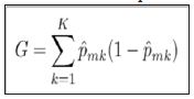
where ˆpmk represents the proportion of training observations in the mth node that come from the kth class.

From inspection, we can see that the Gini index takes on a small value if all of the class proportions are close to zero or one. This can be viewed as a measure of node purity, where a small value indicates that the node predominantly contains observations for a single class.

A popular alternative to the Gini index is cross-entropy, defined by

Equation 2

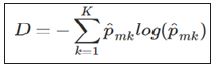
Cross entropy will also take on a value near zero if all of the class proportions are near zero or near one, so it is similar to the Gini index in its interpretation. To build a tree, the algorithm starts with the entire population, which serves as the root node, and then examines a set of variables. The Gini index of the root node is calculated. Subsequently, for each variable being considered, the Gini index of the resulting children nodes is calculated. The variable creating the lowest Gini index is chosen, and the process continues recursively on the children until no improvement can be made. For prediction, an observation starts at the root node and then follows a path down the tree. When it reaches a leaf node, the tree’s prediction is whichever class has the highest proportion.

Equation 3

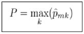
For ensemble models, many trees are generated in this manner, and the final prediction is an aggregation of predictions from all the individual decision trees.

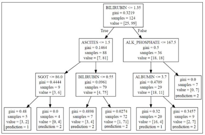
Once a model is made, the question arises on how to interpret the output. For a single decision tree, the actual splitting decisions on variables can be examined to understand relationships. Consider the tree in (Figure 1), built off of the Hepatitis data set. Further description of the data set is discussed in Section 7.1. To understand how a variable improves accuracy, the splits and paths can be explored. For this tree, the variable bilirubin is used to split on two interior nodes, whereas ascites, alk phosphate, sgot and albumin are only used on one interior node. Bilirubin seems to be more important since it was selected by the algorithm twice. Also, the relative location of the variables in the tree can provide a different insight. In general, the higher up in the tree the node is, the bigger the gain in accuracy by splitting. Thus, bilirubin may make a relatively bigger difference on a larger proportion of patients than, for example, sgot, (Figure 1). Lastly, relationships between variables and outcomes can be inferred by examining the final interior nodes. For the bottom leftmost interior node, the split is defined as class 1 (die) if sgot is less than or equal to 86, and class 2 (live) otherwise. However, this interpretation becomes more difficult when examining nodes on higher levels.

Figure 1 : Decision Tree on Hepatitis Data Set.

Understanding a single decision tree is manageable, but as the number of trees increase, this visual understanding quickly becomes intractable. This is currently overcome by generating a measure of average effect over all the trees. Variable importance is defined as the total amount that the Gini index is decreased when it is split over a given variable and averaged over the number of trees [7]. The larger the number, the bigger the effect. A graphical representation of variable importance is presented in (Figure 2). We can infer from the graph that albumin makes the biggest average improvement in node accuracy when splitting, whereas antiviral make hardly any gains when used as splitting variables. Variable importance is valuable to see how well the variable is influencing the structure of the tree, but it does fall short when trying to understand how the variable is important to a given outcome. In this regard, regression models are still superior.

Figure 2 : Random Forest Variable Importance on Hepatitis Data Set.

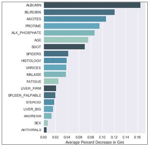
Variable importance as it is defined gives a measure of how well the model is differentiating between classes, but it suffers from two key weaknesses. The first is that it does not measure how a variable influences the target variable; instead, it simply tells us that there is some effect in shaping the tree (Figure 2). The second is that it tends to favor variables that make the biggest overall impact on the model. Since the Gini index is a main component of the calculation, the higher the variable importance is, the more likely the variable is to appear at the top of the tree. This bias in variable importance is known and has been explored in previous studies [14-16] with new ways of reducing the bias presented. Still, there has been little discussion of new measures in the literature.

What we desire is a measure that tells us not that the variable is important, but that it is important for detecting a specific class. For a given class C of a target variable, let c represent the number of training examples in the class. Define the importance of a variable V with respect to the class c over a model with k trees as

Equation 4

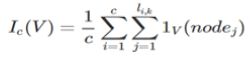
Where li,k represents the length of the path for example iover tree k, and 1V(nodej) being defined as 1 if the variable for nodej equals V and 0 otherwise.

Using Class Variable Importance (CVI), we can begin to understand the variable importance with respect to every class. For example, using the standard variable importance (Figure 2), we can only infer that albumin and bilirubin have a high chance of being at the top of the tree, given their large values. Examining a tree from model (Figure 1), that insight holds true. What would be more useful to know from an action ability standpoint is what variables went into generating a specific path. What variables went into classifying instances falling in the leftmost leaf node? Variable importance alone cannot tell us that.

When looking at the path of a variable ending in the first leaf node on the left, bilirubin, ascites, and sgot all appear in one node in the path. However, when considering the third leaf node from the left, bilirubin is counted twice, being in two path nodes, whereas ascites still appears only once. CVI gives us a way to look at the average of all these paths per class over all the training examples. Looking at the paths for all examples of a given class, we can measure the average number of times a variable is passed through to get to a prediction.

This measure on its own is a step toward better interpretability; the more a class passes through a variable, the more that variable is sifting through nuances in the class behavior. However, the question still exists as to the degree of an effect. If the variable is equally important to all classes, it does not demonstrate a preference toward one class or another. To help give insight into the degree of the effect, we can define pair wise ratios of class importance. For a two class classification problem, where C = [0, 1], we can examine the ratio of importance between classes, or

Equation 5

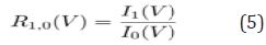
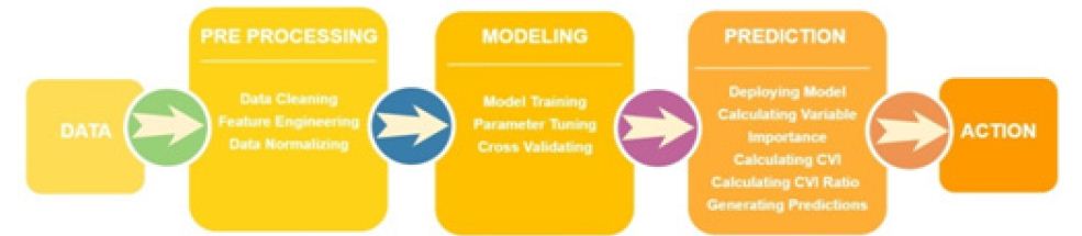
Ratios close to one indicate no real discriminative power, whereas ratios above or below one show preference towards the positive class or negative class respectively. We cannot infer the direction of the relationship as we can with regression models, but we can say that a given variable is more influential for one class or another so that the strength of the discriminative power can be found. It is worth noting that CVI does not change the way models are built-it merely enhances the interpretive power in post analysis. Considering that the traditional machine learning flow consists of processing data, building a model, deploying the model, and using predictions made, it can be argued that the most important part of machine learning occurs at the end of the flow. In the medical setting, the final step, acting on the prediction, can be critical in saving a patient’s life (Figure 3).

Figure 3 : Carcass characteristics of Yak.

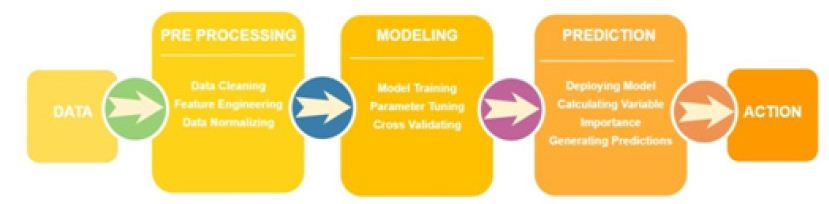
While data cleaning and feature engineering can improve accuracy, without meaningful ways to use the prediction, the effort to build a model is wasted. Thus, more focus should be placed on the prediction phase to help utilize the predictions generated. CVI is calculated on top of all of the modeling that has already been done and can be calculated on any tree-based model. It can be retroactively included in currently deployed models as well as added on to any future modeling work with minimal computational expense. The resulting new measure provides more resources for a medical practitioner to use in their decision making, which can be valuable in generating a holistic view of a given patient (Figure 4).

Figure 4 : Carcass characteristics of Yak.

For pH (1h), the steer and female had similar scores but the bull was significantly higher. For pH (24h), all three sexes were similar but they are higher than would be expected for cattle suggesting that this may have been genetics or the animals may have been stressed before they were harvested. Also in general grass fed animals normally have higher ultimate pH values than grain fed animals (Table 2).

To see how useful class variable importance is in practice, an analysis was done on several benchmark datasets. Exploration of several tree-based methods was employed: Extra Trees (ET), Random Forests (RF), and Gradient Boosted Trees (GBT). Since the variables themselves were of key interest, no feature engineering was performed on the data. For preprocessing, median values were imputed on any missing data, and all numerical variables were normalized. AUC (Area under the Curve) of the ROC (Receiver Operating Characteristic) was chosen as the optimization metric, resulting in one best model of each respective algorithm per dataset.

Hepatitis Data

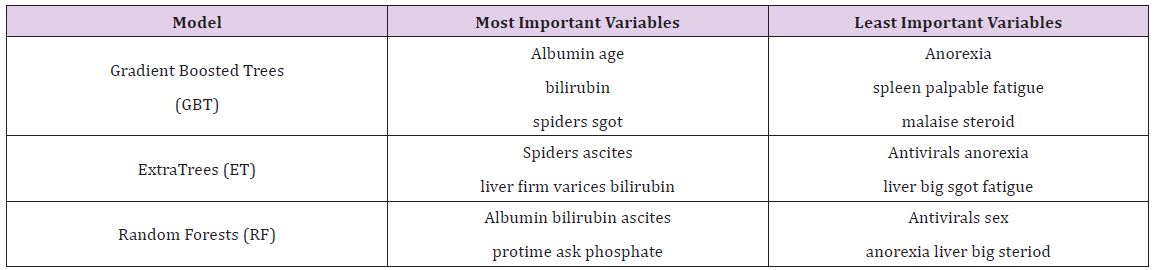
The Hepatitis dataset in this study is from UCI Machine Learning Repository, which included 155 samples with 20 attributes (14 binary, 6 numeric attributes). The objective of this dataset is to identify or predict whether patients with hepatitis are alive or not (1 for die and 2 for live). The model performance for each algorithm is reported in (Tables 1 & 2). Given that Extra Trees has the highest classification accuracy; it may be the favored model in terms of inference, though each model has its strengths and weaknesses to consider before deployment (Table 1). After the models were built, the corresponding variable importance and ratio importance Rlive, die (V) were calculated for each variable. Looking at the ranked lists of overall variable importance in (Figure 2), medical practitioners may make decisions for treatment based on which variables have the largest values. For example, in the Random Forests model, albumin and bilirubin seem most important. Using knowledge on a specific patient, they may go down the ranked list of variables starting with albumin and bilirubin until they find one they can influence for the patient’s situation. They would likely not consider antiviral, since these had the lowest importance of all.

Table 1 : Model Performance for Hepatitis Data.

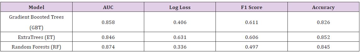
Table 2 : Most and Least Important Variables on Hepatitis Data.

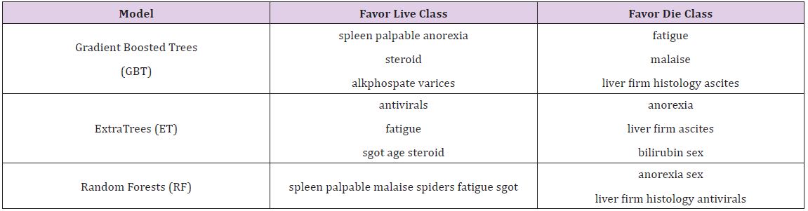
If instead we consider the ratio importance in (Figure 3), we see a very different picture. For the same Random Forests model, ‘spleen palpable’ and ‘malaise’ seem to favor the live class, whereas ‘anorexia’ and ‘sex’ seem to favor the die class.

It is worth noting that antivirals, which had relatively low overall variable importance, demonstrated a significant preference for the die class in the ratio representation. If a patient is given a death prognosis from a model, it may be more valuable in that specific patient’s case to focus on spleen palpable, malaise, anorexia, and sex in trying to bring about a change in the patient’s outcome since those are more strongly favoring one class or another. We cannot determine the direction of the relationship, whether it be negatively or positively correlated, but with domain expertise, this can be inferred. For example, it may be that malaise favors the live class, but that does not imply that the relationship is positive. It may be that when malaise is not present, a live prediction is generated. With domain experience, these types of nuances can be understood with decision making (Table 2).

This inversion of ranking appeared not just with antiviral in the Random Forests model, all models had some low-ranked variable importance appear high when examining the ratio importance. It is worth considering what causes this to be so. For these variables, it is very likely that they often appear at low leaves in the tree. Thus, they do not appear often, but when they do, they exhibit the strongest effect. Consider a dataset with a binary variable that is 0 most of the time. However, whenever it has a value of 1, the same class is always predicted. While the value of 0 may predict either class, the fact that when it is present it predicts 1 is a strong relationship, one that a regression model is more likely to detect. Creating a ranking of importance increases the ability of a tree based model to detect relationships of this sort (Table 3).

Table 3 : Most and Least Important Variables on Hepatitis Data.

Breast Cancer Data

The Breast Cancer dataset in this study is from UCI Machine Learning Repository, which included 569 samples with 32 attributes (all numeric attributes). The objective of this dataset is to identify or predict whether the cancer is benign or malignant (M for malignant and B for benign). The model performance for each algorithm is reported (Table 4). Given that all models demonstrate the same classification accuracy and relatively similar AUC, the best model may be the Gradient Boosted Trees with the lowest Log Loss. Yet, each model has its strengths and weaknesses to consider before deployment (Table 5).

Table 4 : Model Performance for Hepatitis Data.

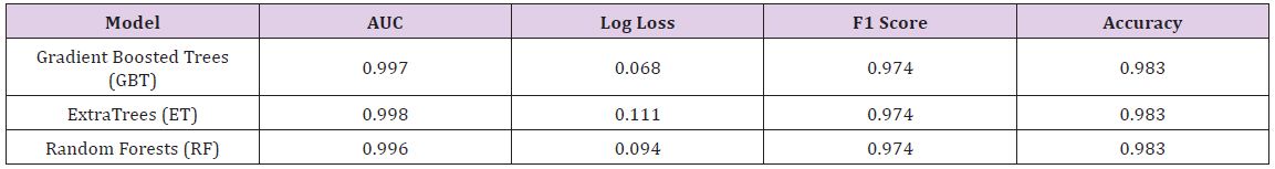
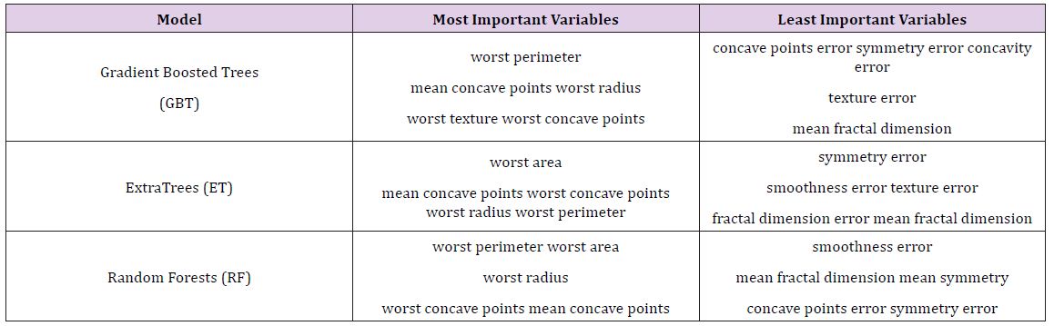
Table 5 : Most and Least Important Variables on Breast Cancer Data.

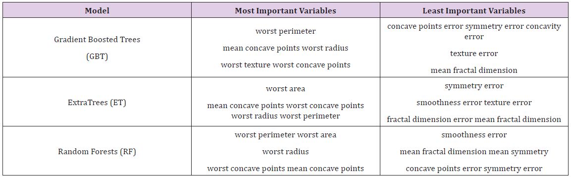
After the models were built, the corresponding variable importance and ratio importance RB, M (V) were calculated for each variable. Looking at the overall variable importance in (Table 5), we see the same set of variables appearing important across all models: ‘mean concave points,’ ‘worst concave points,’ and ‘worst radiuses. Given that the models had similar performance metrics, this is not surprising, and we can be more confident that these variables are truly important for a large portion of the examples in the training data. But again, we do not know why these variables are important, just that there seems to be some value in the ‘mean concave points,’ ‘worst concave points,’ and ‘worst radiuses when discriminating between benign and malignant tumors (Table 5).

When examining the ratio importance in (Table 6) however, more variation is present between models. ‘Symmetry error’ is most strongly related to the Extra Trees and Random Forest model, whereas ‘radius error’ is most important for Gradient Boosted Trees. In this situation, we see the same inverse presentation in the variable ranking as is witnessed in the hepatitis data: the least important variable in the Extra Trees and Random Forests model, ‘symmetry error’, and now has the strongest effect in the ratio representation. Again, this suggests that while it may not impact the majority of instances, when it does appear at the lower branches of the tree, the differences between classes are notable. When looking for innovation in cancer treatment, new ways of looking at the same data are needed to stimulate novel ideas.

Table 6 : Ratio Variable Importance on Breast Cancer Data.

Class Variable Importance (CVI) presents a new way of interpreting variable relationships in tree-based models. The fact that both datasets presented very opposing views of certain variables demonstrates the importance of considering different measures of variable importance: what is apparent in one representation is not always apparent in another, and in such a domain as medicine, that new representation may provide hidden insight. It is likely that the variable is only present in the bottom most splits of the trees, indicating that while not used often, for those instances where it is used, the variable is the biggest differentiator between the classes (Table 6).

CVI presents a very different interpretation of the variable relationship than the top down approach of standard variable importance. The commonly used variable importance measure is insightful in that it measures how strongly variables influence a lot of training instances; being a measure of how likely the variable is to appear in a top split of a tree and not how much it influences a specific prediction. CVI tries to overcome this by measuring the strength of the effect with respect to each class. If the class variable importance is relatively the same between all classes in the target variable, it can be inferred that the variable favors all classes similarly. To represent this relationship more cleanly, a ratio of class variable importance can be calculated, with ratios greater or less than one inferring that the variable favors one class over another. When looking for actionable model results by decision makers, as is often the case in the medical domain, this representation gives more useful information than variable importance on its own.

The fact that CVI measures the relative effect of a variable between classes and is not weighted by the proportion of nodes in the tree allows for the detection of more nuanced relationships. However, if the goal is to find variables with high relationships and a large portion of classes, a holistic look at the feature importance can be employed. Variables that have both high variable importance and high ratio importance can be identified as having affecting many examples and in the same way. It may not be easy to infer the direction of the relationship, but by looking at patients on a case by case basis and applying domain expertise, variables can be identified that are influential to a given example and its class prediction. While it is difficult for a single measure to convey a complete picture of a data set, creating a variety of measures to represent different nuances is key to better understanding and insight. In this regard, further exploration of variable importance in regard to inference is essential. Exploring different approaches for calculating the variable effect within the trees may result in more useful measures. For example, employing the Gini index instead of an indicator function or incorporating the actual splitting rule on the nodes into the class importance calculation may present the variables differently. Devising a weighting scheme to give more credence to importance ratios with a larger proportion of nodes in the tree may make detecting variables influencing a larger portion of the population. In future work, we plan to explore these nuances further.

This work was conducted under no financial support of any kind. To our knowledge, there are no potential conflicts of interest in the work being presented. Thank you to Damian Mingle and the Analytics Division of Intermedix for their support and encouragement in pursuing this research.

1. Kellie J Archer, Ryan V Kimes (2008) Empirical characterization of random forest variable importance measures. Computational Statistics & Data Analysis 52(4): 2249-2260.
2. JH Olshen, RA Stone, CJ Breiman, Leo Friedman (1984) Classification and Regression Trees. Chapman and Hall/CRC, USA.
3. Leo Breiman (2001) Random forests. Machine Learning 45(1): 5-32.
4. Alexandre Bureau, Jos´ee Dupuis, Kathleen Falls, Kathryn L Lunetta, Brooke Hayward, et al. (2005) Identifying snps predictive of phenotype using random forests. Genetic epidemiology 28(2): 171-182.
5. Xi Chen, Hemant Ishwaran (2012) Random forests for genomic data analysis. Genomics 99(6): 323-329.
6. J Friedman (2001) Greedy function approximation: A gradient boosting machine. The Annals of Statistics 29(5): 39.
7. Jerome Friedman, Trevor Hastie, Robert Tibshirani (2001) The elements of statistical learning. Springer series in statistics New York, USA.
8. Robin Genuer, Jean Michel Poggi, Christine Tuleau Malot (2010) Variable selection using random forests. Pattern Recognition Letters 31(14): 2225-2236.
9. Pierre Geurts, Damien Ernst, Louis Wehenkel (2006) Extremely randomized trees. Machine Learning 63(1): 3-42.
10. Silke Janitza, Carolin Strobl, Anne Laure Boulesteix (2013) An aucbased permutation variable importance measure for random forests. BMC bioinformatics 14(1): 119.
11. Kathryn L Lunetta, L Brooke Hayward, Jonathan Segal, Paul Van Eerdewegh (2004) Screening large-scale association study data: exploiting interactions using random forests. BMC genetics 5(1): 32.
12. JR Quinlan (1986) Induction of decision trees. Machine Learning 1(1): 81-106.
13. J Ross Quinlan (2014) C4. 5: programs for machine learning. Elsevier, USA.
14. Marco Sandri, Paola Zuccolotto (2008) A bias correction algorithm for the gini variable importance measure in classification trees. Journal of Computational and Graphical Statistics, 17(3): 611-628.
15. Carolin Strobl, Anne Laure Boulesteix, Thomas Kneib, Thomas Augustin, AchimZeileis (2008) Conditional variable importance for random forests. BMC bioinformatics 9(1): 307.
16. Carolin Strobl, Anne Laure Boulesteix, Achim Zeileis, Torsten Hothorn (2007) Biasin random forest variable importance measures: Illustrations, sources and a solution. BMC bioinformatics 8(1): 25.